The Transformer Architecture: Encoder versus Decoder

12 Aug 2026 · 7 min read

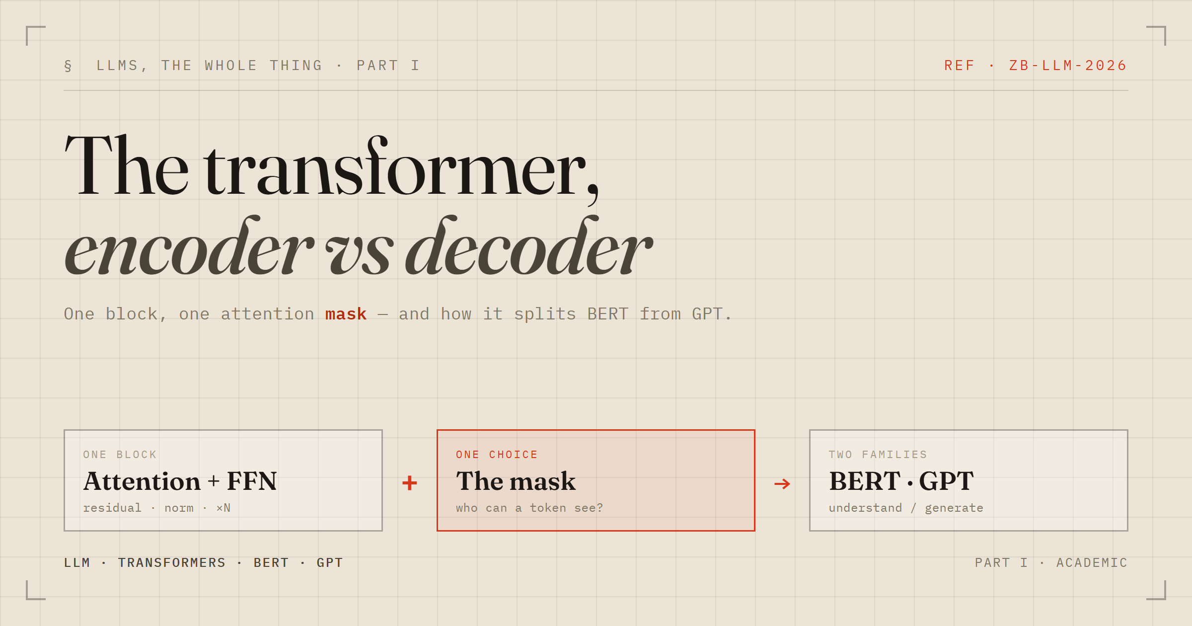
The transformer, introduced in 2017 in Attention Is All You Need, underpins essentially every modern large language model. Yet the family it spawned is not uniform: BERT, GPT and T5 are all transformers, and they behave very differently. This article — the first in a series that works through LLMs from the ground up — establishes the single distinction from which almost everything else follows. It is not the size of the model, nor the training data, nor the number of layers. It is a choice about which tokens a given position is allowed to attend to: the attention mask.

One block, repeated

A transformer is a stack of identical layers. Each layer performs two operations in sequence. First, self-attention lets every token gather information from other tokens; this is the only point in the layer where positions exchange information. Second, a position-wise feed-forward network transforms each token independently. Both operations are wrapped in residual connections and layer normalisation, which is what allows the stack to be made deep without the gradients degrading.

Everything that distinguishes an encoder from a decoder lives inside the first operation. The feed-forward network, the residuals, the normalisation, the overall shape of the tower — these are shared. So the question “encoder or decoder?” is really a question about how self-attention is constrained.

Self-attention, briefly

Self-attention projects each token into three vectors: a query, a key and a value. The relevance of token j to token i is the dot product of i’s query with j’s key. Those scores are scaled, passed through a softmax so that each row becomes a probability distribution, and used to take a weighted average of the value vectors. The output for each token is therefore a blend of the tokens it attended to.

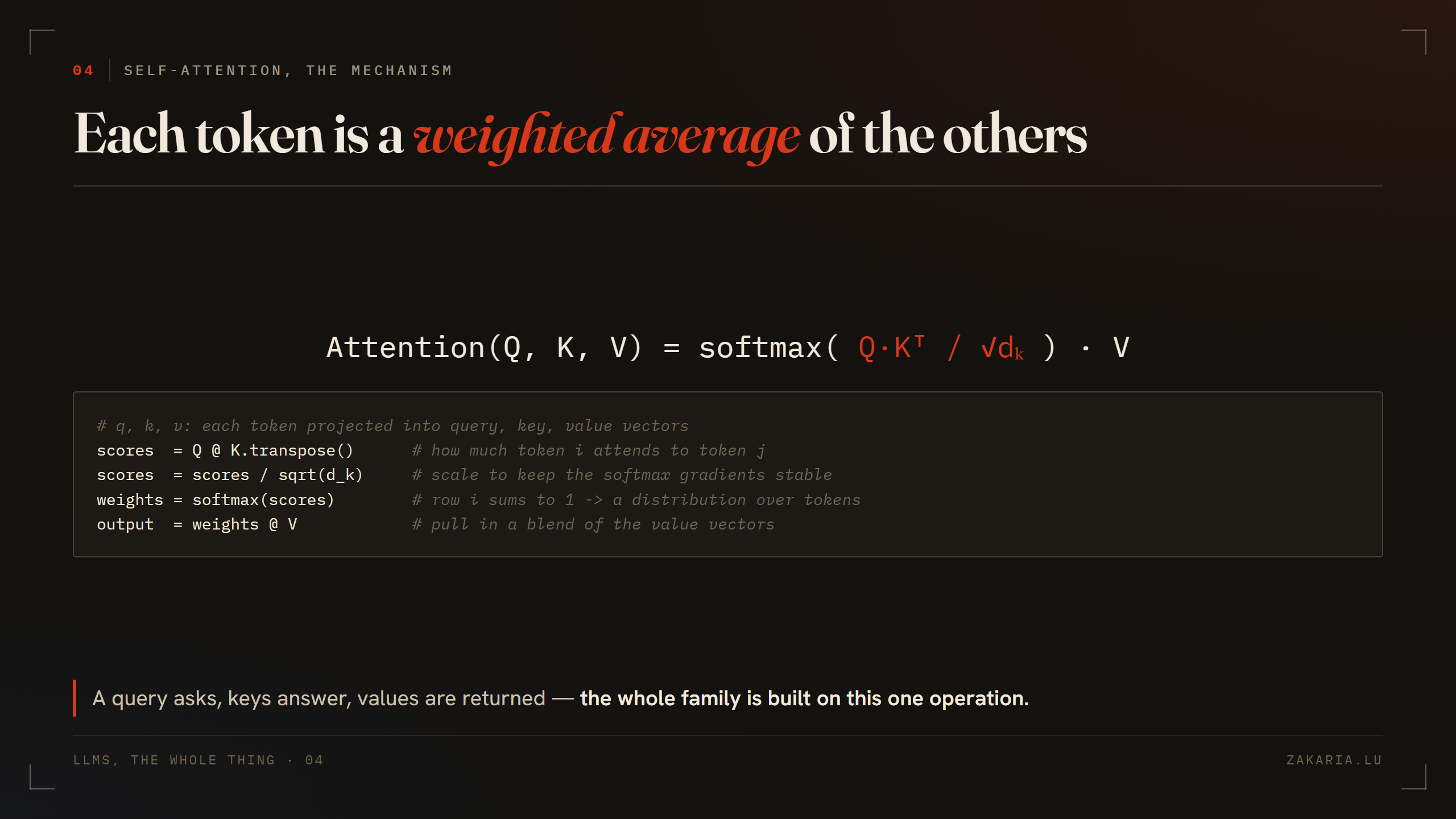
The scaled dot-product attention formula, Attention(Q,K,V) = softmax(QKᵀ/√dₖ)V, with four lines of pseudocode computing scores, scaling, softmax and the weighted sum of values. — Scaled dot-product attention: a query asks, keys answer, values are returned. Every transformer variant is built on this one operation.

The crucial detail for what follows is the softmax step. Because the weights are produced by a softmax, any score set to negative infinity before the softmax receives a weight of exactly zero afterwards. That is the mechanism by which a token can be forbidden from attending to another: not by removing it, but by driving its score to −∞. The mask is simply a matrix of which scores get that treatment.

The decisive choice: the mask

Two masks matter. A bidirectional (unmasked) attention pattern lets every token attend to every other token, to its left and to its right. A causal mask permits token i to attend only to tokens 0 through i — the future is hidden.

Two attention matrices for the sentence 'the cat sat on'. The bidirectional matrix is fully ticked; the causal matrix is lower-triangular, with the upper-right cells masked out in red. — The same attention, two masks. The causal pattern is lower-triangular — a token can never read a position that comes after it.

This is the whole distinction. An encoder uses bidirectional attention. A decoder uses causal attention. The two are otherwise the same network; one can be turned into the other by adding or removing a triangular mask. Every downstream difference — how the model is trained, what it produces, what it is good for — is a consequence of whether the future is visible.

Two ways to train the same block

The distinction becomes concrete at training time. Take a single sentence — “This is an example of how concise I can be” — and present it to each model the way its objective demands. The preprocessing is identical: the text is tokenised and embedded before it ever reaches the stack. What differs is the shape of the input and the question being asked of the output.

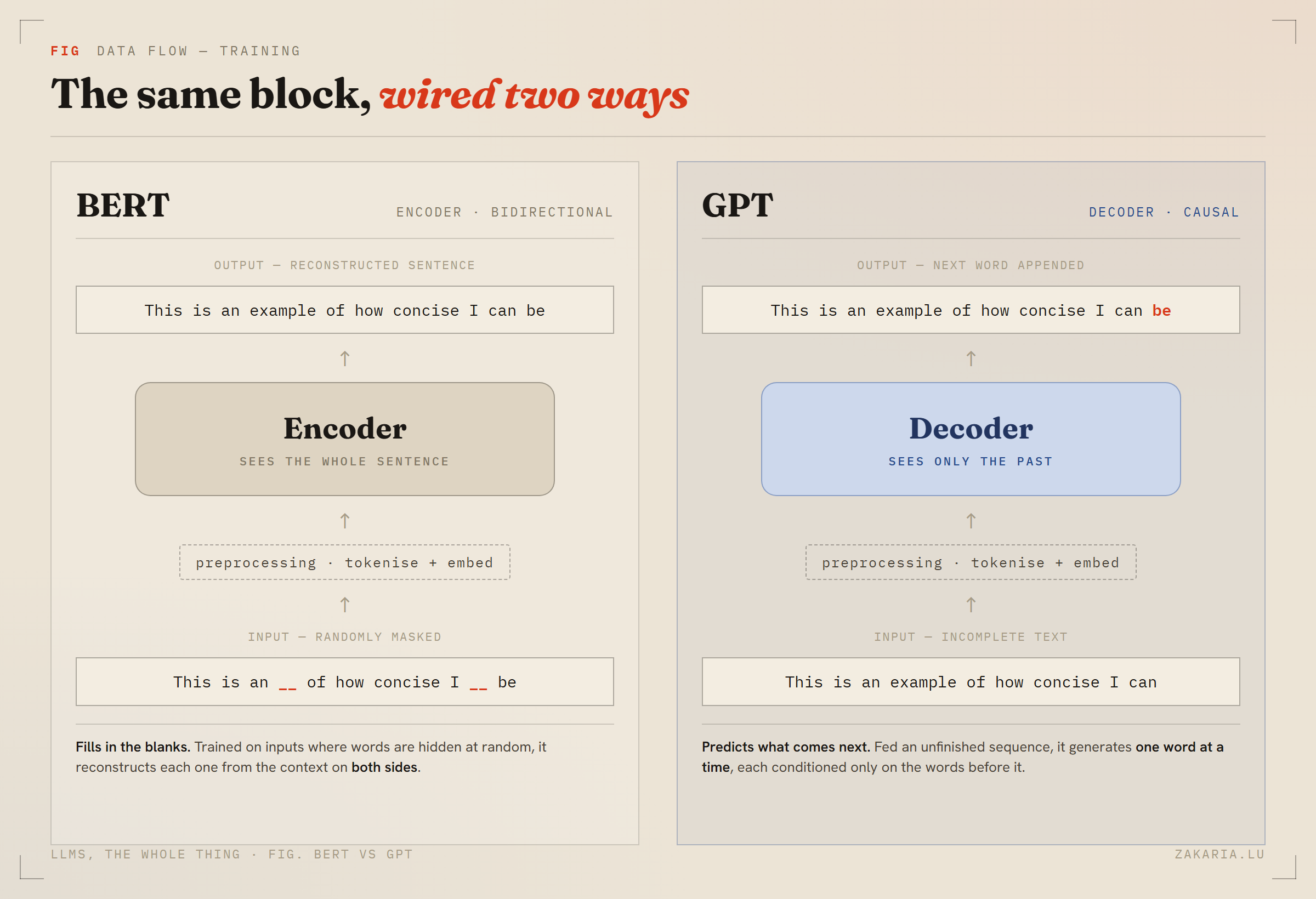
Two side-by-side pipelines for the sentence 'This is an example of how concise I can be'. Left, BERT: a masked input with two blanked words flows up through preprocessing into a grey Encoder box and out as the fully reconstructed sentence. Right, GPT: an incomplete input ending at 'I can' flows up through preprocessing into a blue Decoder box and out as the sentence with the next word 'be' appended. — The same tokenised input, two training regimes. BERT restores masked words using both sides; GPT extends an unfinished sequence one word at a time using only the left.

The encoder is shown the sentence with words blanked out and must restore them. Concretely, some tokens are replaced by a special [MASK] placeholder, and the model predicts what belonged in each slot:

input    →  This is an [MASK] of how concise I [MASK] be
predict  →  [MASK]₁ = "example"     [MASK]₂ = "can"

To recover a blank the model may read everything around it, including the words that come after — which is precisely why bidirectional attention is mandatory here rather than merely convenient.

The decoder never sees a blank. It is shown a prefix that stops partway and must produce only the next token, using nothing but the words that came before:

input    →  This is an example of how concise I can
predict  →  next token = "be"

The sentence is therefore generated left to right, one token at a time. Same preprocessing, same stack of blocks — only the mask, and therefore the task, differs.

Encoders: built to understand

The canonical encoder is BERT. Because it sees context on both sides, it is trained with masked language modelling: roughly 15% of tokens are hidden and the model reconstructs them from everything else in the sentence. Bidirectional context is not a convenience here; the objective requires it, since reconstructing a hidden token from both neighbours is only possible if both neighbours are visible.

An encoder does not generate text. It emits a contextual vector for every input token, and a small task-specific head is attached on top for classification, sentiment analysis, named-entity recognition, extractive question answering, or the sentence embeddings used in semantic search. The encoder’s strength is representation: it consumes a complete input and produces an understanding of it.

Decoders: built to generate

The canonical decoder is GPT. Its causal mask makes next-token prediction a well-posed objective at every position simultaneously: predict token i+1 from tokens 0..i. Because no position can see its own target, the model can be trained on every position of a sequence in a single forward pass without leaking the answer — the property that makes decoder pre-training so efficient at scale.

Generation is then autoregressive: the model emits one token, appends it to the input, and predicts the next. A key–value cache stores the keys and values of past tokens so that each new step is cheap rather than a full recomputation. This is why the modern generative LLM — the thing that writes prose, code and dialogue — is a decoder.

Encoder–decoder: reading one thing to write another

The original 2017 transformer used both halves. An encoder reads a source sequence bidirectionally; a decoder generates a target sequence causally; and a third attention mechanism, cross-attention, connects them. In cross-attention the decoder supplies the queries while the encoder’s output supplies the keys and values, so the generator can look back at a fully understood source as it writes.

A schematic: a bidirectional encoder on the left connected by cross-attention to a causal decoder on the right, with two cards explaining cross-attention and its sequence-to-sequence use cases. — Cross-attention is the bridge from understanding to generation — the decoder’s queries read the encoder’s keys and values.

This shape suits sequence-to-sequence tasks where the input and output are distinct, such as translation and summarisation. T5 generalises the idea by framing every task as text-to-text.

Choosing an architecture

The three shapes map cleanly onto three kinds of problem. Reach for an encoder when you hold the whole input and want to classify, tag or embed it. Reach for a decoder when you need to produce text. Reach for an encoder–decoder when a distinct source must be transformed into a distinct target.

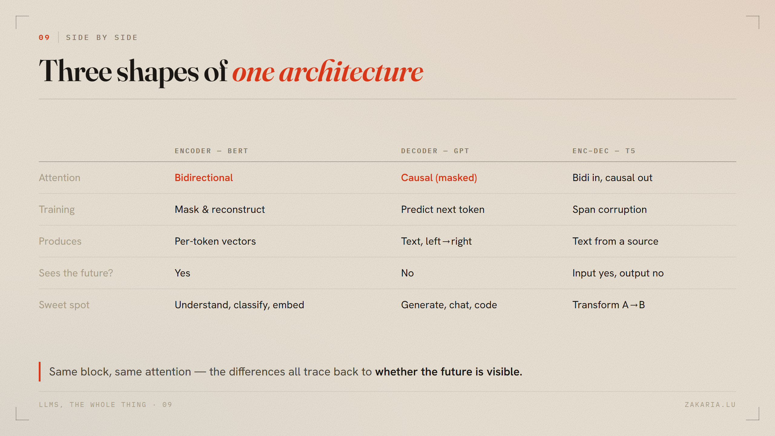
A comparison table of encoder (BERT), decoder (GPT) and encoder-decoder (T5) across attention type, training objective, output, whether the future is visible, and sweet spot. — Three shapes of one architecture. Every row traces back to a single variable: whether a token can see the future.

It is worth holding the summary in mind as a single sentence. BERT reads the whole room; GPT writes one word at a time and cannot see ahead. Both are the same transformer block; the difference is the mask.

What comes next

Establishing the encoder–decoder distinction leaves several mechanisms deliberately unopened. Subsequent articles in this series will look inside multi-head attention — why attention is split into several parallel heads rather than computed once — and at positional encodings, which are what let an otherwise order-agnostic operation know that “the cat sat” is not “sat the cat”. From there the path leads to how these blocks are actually trained, and to the design decisions that separate one generation of model from the next.