Causal attention and the two masks: one hides the future, one cuts links on purpose

7 Sep 2026 · 6 min read

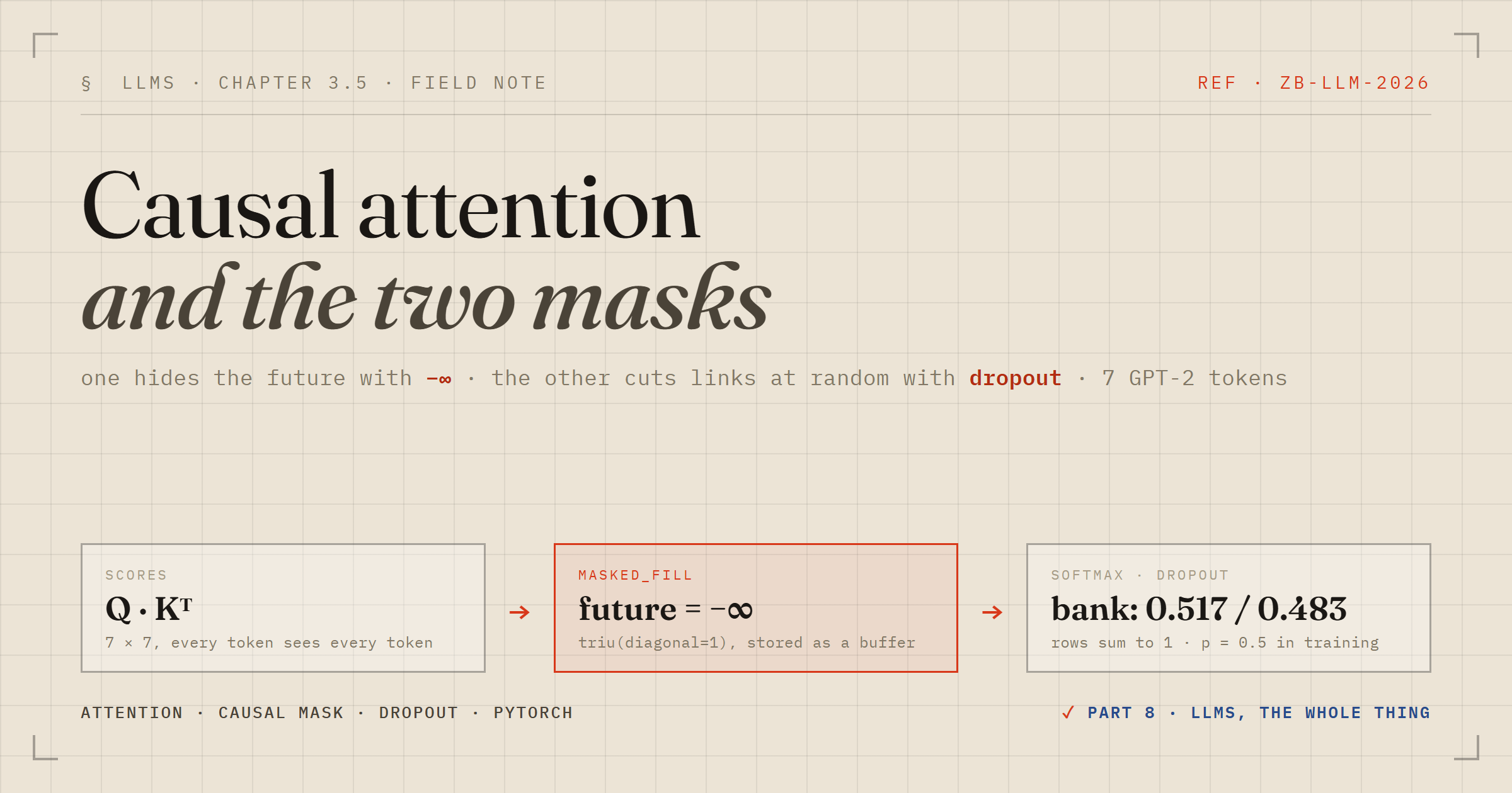
Section 3.5 of Raschka's Build a Large Language Model (From Scratch) adds three things to the single attention head from section 3.4: a mask that stops a token looking at the tokens after it, dropout on the attention weights, and a batch dimension. The mask is the one that changes what the model is. Dropout is a second mask that only exists while training. This post is the section worked end to end on the same seven GPT-2 tokens I used last time, The bank of the river was muddy, with every matrix taken from a real run at seed 123. The slides in this post are from the deck I built from the same notes.

The problem: “bank” is reading words that do not exist yet

Plain self-attention lets every row of the 7 × 7 weight matrix spend probability on every column. Here is the row for bank from the section 3.4 head:

          The   bank     of    the  river    was  muddy
  bank  0.154  0.144  0.141  0.144  0.139  0.138  0.140

Seventy percent of that row goes to the five tokens after “bank”. For a model whose job is to predict the next word, that is the answer leaking into the input. When GPT is asked what follows “The bank”, the words “of the river was muddy” have not been generated yet. Train with the leak and the model learns a trick it can never use at inference.

The fix has one rule: a row may only use columns at or before itself. Rows are the token doing the looking; columns are the tokens being looked at. Everything below is about where in the pipeline to enforce that rule.

The naive mask breaks the row sums

The obvious first move is a lower-triangular matrix of ones from torch.tril, multiplied element-wise into the attention weights. It zeroes the future. It also breaks something.

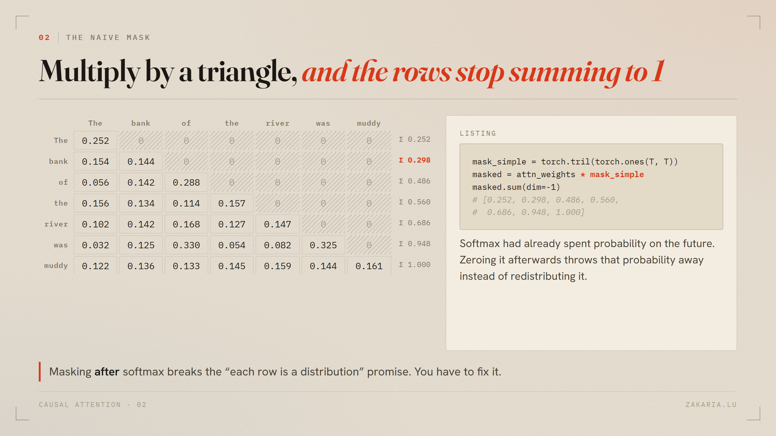
Seven by seven attention weights after multiplying by a lower-triangular mask, with future cells hatched and a row-sum column showing 0.252, 0.298, 0.486 and so on instead of 1. — The future is gone, but the row for “bank” now sums to 0.298. Softmax had already spent that missing 0.702 on the five hidden tokens.

The rows were probability distributions before the multiply and are not afterwards. The book's first repair is honest: sum each row and divide by it. That gives “bank” a 0.517 / 0.483 split over the two tokens it is allowed to see, and every row sums to 1 again.

row_sums = masked_simple.sum(dim=-1, keepdim=True)
masked_simple_norm = masked_simple / row_sums
# bank  0.517  0.483  0.000  0.000  0.000  0.000  0.000

Correct, but it is three operations where one would do, and the future took part in the softmax denominator before being thrown out. It is a leak followed by a patch.

Put −∞ on the scores, then run softmax once

The trick that production code uses relies on one property of softmax: e−∞ is exactly 0. So instead of masking the weights after softmax, mask the raw scores before it. Any cell that holds −∞ contributes nothing to the denominator and comes out as a clean zero.

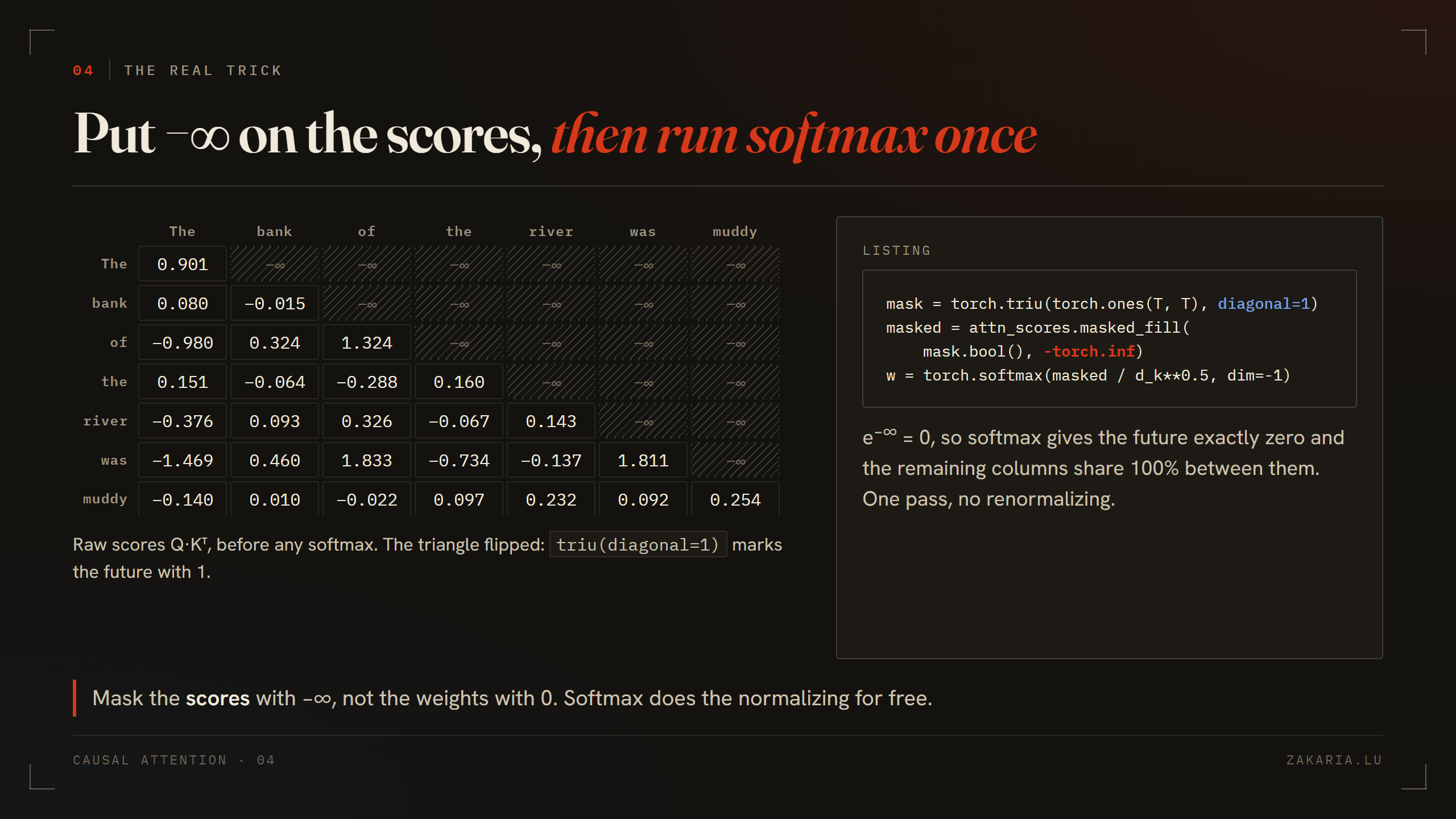
Dark slide with the seven by seven raw score matrix, future cells showing minus infinity, next to the three-line PyTorch listing using triu with diagonal one and masked_fill with minus torch.inf. — Applied to the scores, not the weights. The triangle flips: triu with diagonal=1 marks the future with a 1, and those cells receive −∞.

mask   = torch.triu(torch.ones(T, T), diagonal=1)   # 1 = future
masked = attn_scores.masked_fill(mask.bool(), -torch.inf)
attn_weights = torch.softmax(masked / keys.shape[-1] ** 0.5, dim=-1)

Two details tripped me on first read. The mask is now the opposite triangle from the naive version: tril marked what to keep, triu(diagonal=1) marks what to hide. And diagonal=1 matters: without it the diagonal itself would be hidden and a token could not attend to itself.

I compared the two routes on the same head. The largest difference between the renormalized naive matrix and the −∞ matrix was 2.98 × 10⁻⁸, float32 noise. Same maths, leak removed, two operations fewer.

Dropout: the second mask, and it doubles the survivors

Dropout zeroes a random fraction of values and scales the rest by 1/(1−p), so the expected value of each cell is unchanged. Applied to the attention weights it stops the head from leaning on one particular link. The book uses p = 0.5 so the effect is visible; GPT-2 uses about 0.1.

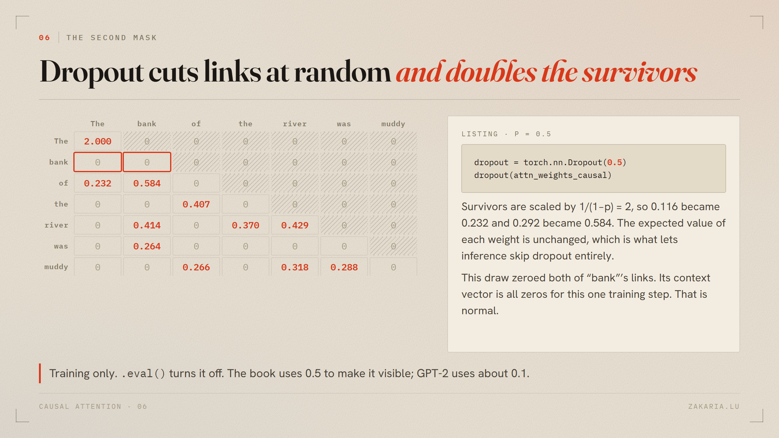
Seven by seven causal attention weights after dropout at p equals 0.5: survivors in red such as 2.000, 0.232 and 0.584, many cells zeroed, and the entire row for bank zeroed. — Survivors doubled: 0.116 became 0.232 and 0.292 became 0.584. This draw cut both of “bank”'s links, so its context vector is all zeros for this one training step. That is normal.

The scaling is what makes inference cheap. Because the average weight is the same with or without dropout, model.eval() simply switches it off and nothing downstream needs to compensate.

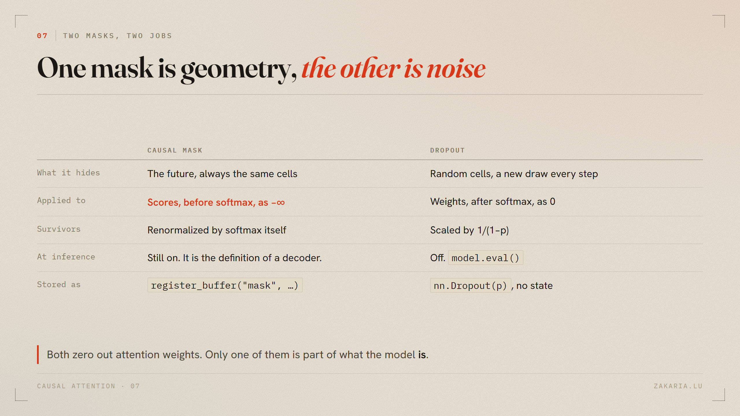
Two masks, two jobs

Both operations zero out attention weights, and I found it useful to write down exactly how they differ, because only one of them is part of what the model is.

Comparison table of the causal mask and dropout across five rows: what it hides, applied to, survivors, at inference, stored as. — The causal mask is applied to scores as −∞ and stays on at inference. Dropout is applied to weights as 0, scales survivors, and is off at inference.

The module: a batch axis and a buffer

Two changes turn the section 3.4 class into CausalAttention. The input gains a batch dimension, so shapes become (batch, tokens, d_in) and the transpose has to name its axes: keys.transpose(1, 2) instead of .T. And the mask is stored with register_buffer.

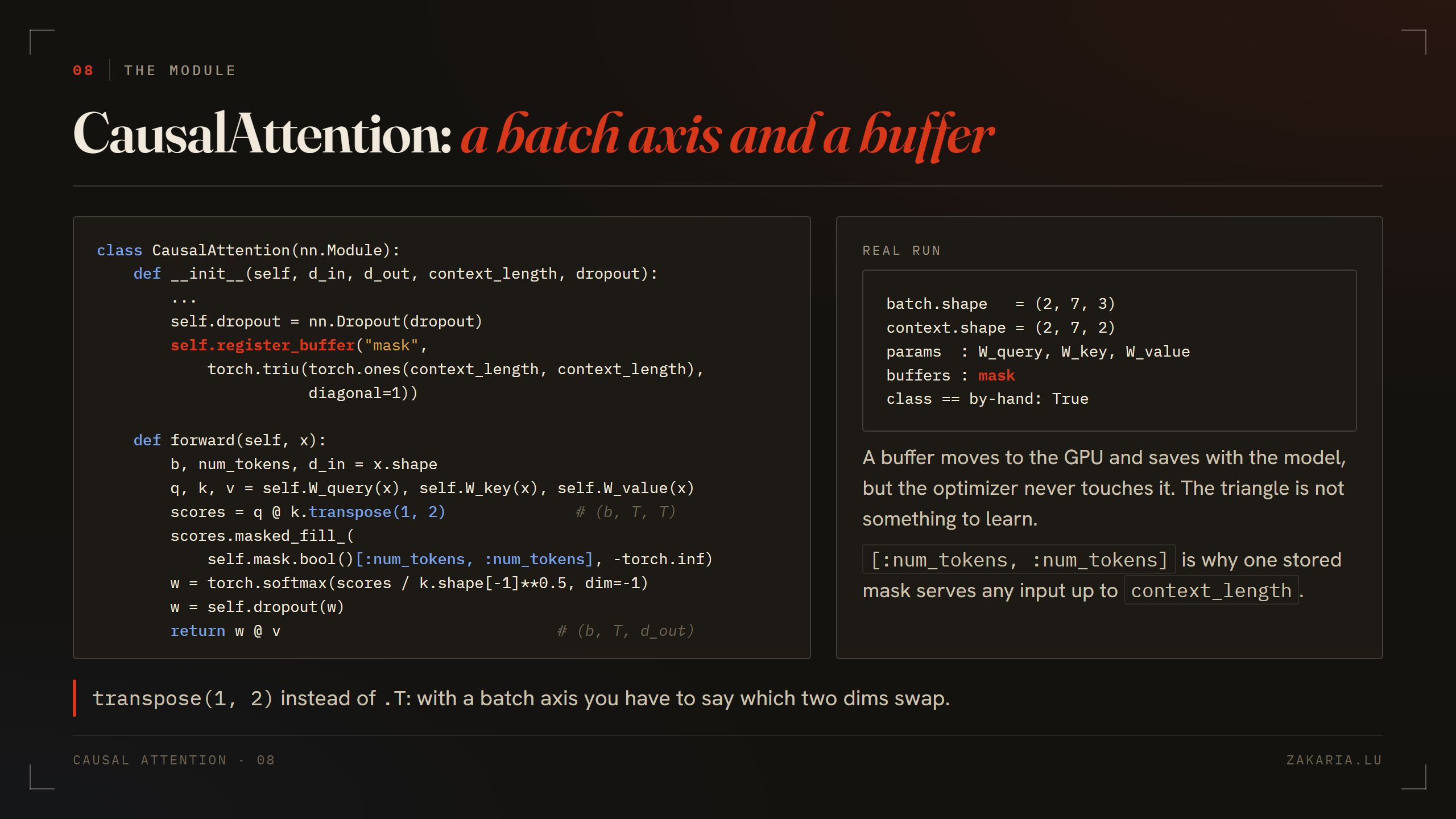
Dark slide with the CausalAttention PyTorch class next to a real-run panel: batch shape 2 by 7 by 3, context shape 2 by 7 by 2, trainable params W_query, W_key, W_value, buffers mask, class equals by-hand True. — A buffer moves to the GPU and saves with the model, but the optimizer never touches it. The triangle is geometry, not something to learn.

The slice self.mask.bool()[:num_tokens, :num_tokens] is why one stored mask of size context_length serves any shorter input: a 7-token batch uses the top-left 7 × 7 corner. And masked_fill_ with the trailing underscore is in-place on the scores, which is fine because the raw scores are not needed after masking and it saves a copy of a (b, T, T) tensor per head.

I checked the class against the by-hand computation with dropout at 0. Identical output, and the module reports exactly three trainable parameters and one buffer.

The whole section in five lines

scores  = Q @ K.T
scores[future] = -inf                   # triu(diagonal=1), a buffer
weights = softmax(scores / sqrt(d_k))   # -inf -> 0, rows still sum to 1
weights = dropout(weights)              # training only, survivors x 1/(1-p)
context = weights @ V

Three things I would tell myself before starting: mask the scores with −∞, not the weights with 0, and let softmax normalize; dropout is a random mask that scales survivors so inference can skip it; and the causal mask is a buffer, saved and moved with the model, never trained.

Repo, walkthrough script, interactive study page and the deck: github.com/zakariahere/chap3-causal-attention. The walkthrough prints every matrix in this post; the deck is in the deck/ folder.