Large Language Models, From the Ground Up - Part I: The Geometry of Meaning

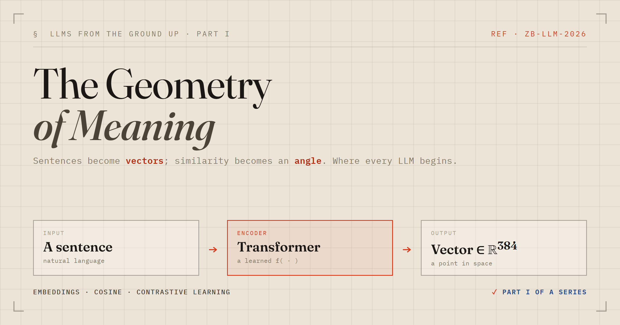
This is the first part of a series that builds up large language models from first principles — not the API-consumer view, but the mechanics underneath. Before attention, before transformers, before a single token is predicted, there is one idea the whole field rests on: turning language into vectors, so that meaning becomes geometry. Get this right and everything above it — retrieval, RAG, multimodal models, the LLM itself — is a variation on the same theme. So that is where Part I starts.

What an embedding actually is

An embedding is a function f: x → ℝd that maps a piece of data to a list of d real numbers, chosen so that geometric closeness approximates semantic closeness. That single sentence carries the entire load. A vector is a point — equivalently, an arrow from the origin — in a d-dimensional space, and the arrangement of those points is learned, never designed. Nobody decides that dimension 47 encodes "royalty" or dimension 112 encodes "plural". The training process simply positions points so that useful relationships fall out of the geometry.

Two properties matter for everything that follows. First, the space is high-dimensional: the model I use below produces d = 384. Second, for most modern text encoders the output vectors are L2-normalised — every arrow has length one and lives on the surface of a unit sphere. That normalisation is not cosmetic; it is what lets us treat direction, and only direction, as the carrier of meaning.

The geometry: similarity is an angle

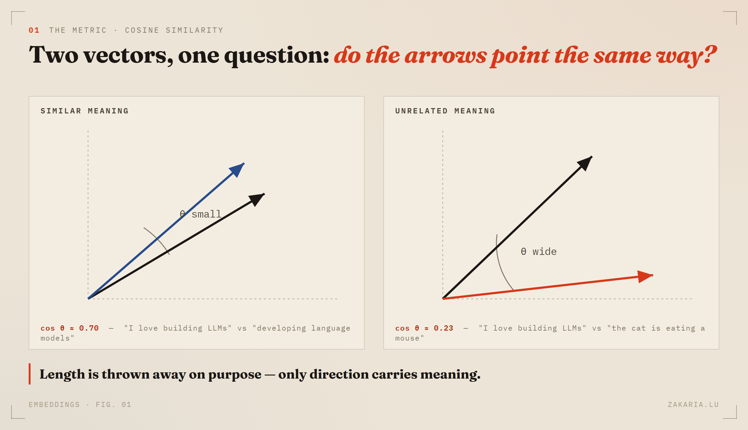
If meaning is direction, then comparing two meanings is comparing two directions — and the natural measure of that is the angle between them. The tool is the dot product (also called the scalar or inner product), which collapses two vectors into a single number. It connects to the angle through one identity worth memorising:

a · b = ‖a‖ ‖b‖ cos θ

Rearranged, cosine similarity is just the dot product with the magnitudes divided out: cos θ = (a · b) / (‖a‖ ‖b‖). And here is the payoff of normalisation: when both vectors already have length one, the denominator is one, so the raw dot product is the cosine. The two are literally the same number. That is why the similarity function in the script below is a one-line np.dot and nothing more.

The value lives in [-1, 1]: 1 means the arrows point the same way (identical meaning), 0 means they are orthogonal (unrelated), -1 means they oppose. A vector compared with itself scores exactly 1 — a zero-degree angle — which makes a useful sanity check.

How the space is learned: contrastive objectives

A space this well-behaved does not appear by accident. It is produced by a loss function that pulls related things together and pushes unrelated things apart. The dominant recipe is contrastive learning. Given an anchor A, a matching positive B⁺, and a batch of negatives, the model is trained to score the true pair highest. The workhorse is the InfoNCE loss, which is nothing more exotic than a softmax classification — "pick the real match out of the crowd" — with a temperature term controlling how sharply the space separates neighbours from strangers.

The consequence is subtle but important: the resulting scores are relative, not absolute. The model is optimised so that a true pair outranks the batch, not so that unrelated items hit exactly zero. Keep that in mind when reading real numbers — which we can now do.

A live run: forty lines of Python

Theory is cheap. Here is the whole pipeline as a self-contained script — it installs fastembed if missing, downloads a small embedding model on first run, embeds four sentences, and computes similarities by hand. The model defaults to BAAI/bge-small-en-v1.5, which is English and emits normalised 384-dimensional vectors, so the dot product is already cosine similarity.

import sys
import subprocess
import numpy as np

# === Step 1: Check and install fastembed ===
try:
    from fastembed import TextEmbedding
except ModuleNotFoundError:
    print("Installing fastembed...")
    subprocess.check_call([sys.executable, "-m", "pip", "install", "fastembed"])
    from fastembed import TextEmbedding

# === Step 2: Load the model (it downloads itself automatically) ===
model = TextEmbedding()

# === Step 3: Define the sentences ===
sentences = [
    "I love building LLMs from scratch.",
    "I really enjoy developing language models.",
    "The cat is eating a mouse in the kitchen.",
    "The car drives fast on the highway.",
]

# === Step 4: Generate the embeddings ===
embeddings = list(model.embed(sentences))  # a list of numpy vectors
print(f"{len(embeddings)} vectors, dim {len(embeddings[0])}")

# === Step 5: Similarity = dot product (cosine, since vectors are normalised) ===
def similarity(vec1, vec2):
    return np.dot(vec1, vec2)

# === Step 6: Pairwise similarity matrix ===
for i in range(len(sentences)):
    for j in range(i + 1, len(sentences)):
        sim = similarity(embeddings[i], embeddings[j])
        print(f"{i+1} <-> {j+1}: {sim:.4f}")

# === Step 7: Semantic search ===
query = "AI and language models"
query_embedding = list(model.embed([query]))[0]

best_score, best_sentence = -1.0, ""
for sentence, emb in zip(sentences, embeddings):
    score = similarity(query_embedding, emb)
    if score > best_score:
        best_score, best_sentence = score, sentence

print(f"closest: {best_sentence!r}  ({best_score:.4f})")

Four sentences: two are about building language models phrased with almost no shared vocabulary ("building LLMs from scratch" versus "developing language models"), and two are unrelated distractors about a cat and a car. Running it produces the scoreboard below.

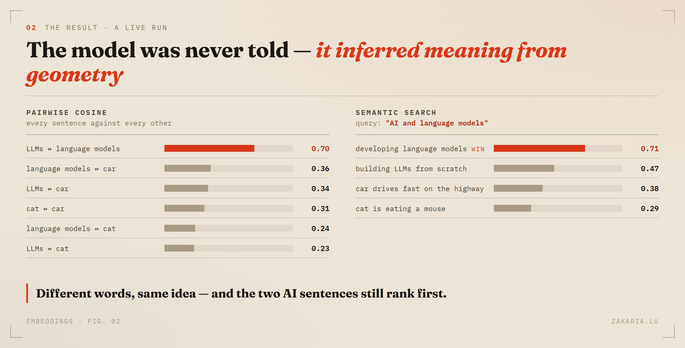
Two things deserve emphasis. The unrelated pairs do not land at zero — they cluster around 0.23 to 0.36, because all English text shares some structure and, as noted, contrastive training optimises ranking, not absolute magnitude. What matters is the gap: 0.70 versus 0.30 is a clean, unambiguous separation. And the semantic search never inspects the raw value at all — it simply picks the largest. That ten-line loop, ranking by cosine, is a functioning semantic search engine.

From one space to many: aligning modalities

Everything so far lives in a single text space. The leap that makes the last few years feel like science fiction is putting different modalities — images, audio, video — into one shared space, so that a picture of a cat and the words "a cat" land near each other. The trick is smaller than it sounds: use a separate encoder per modality, but train them to agree on a shared destination, using naturally paired data.

CLIP is the canonical example. Take a batch of (image, caption) pairs, encode images with a vision transformer and captions with a text transformer, and build the full grid of image-to-caption similarities. The diagonal holds the true pairs; everything off-diagonal is a mismatch. The objective — InfoNCE again, run in both directions — pulls the diagonal up and pushes the rest down.

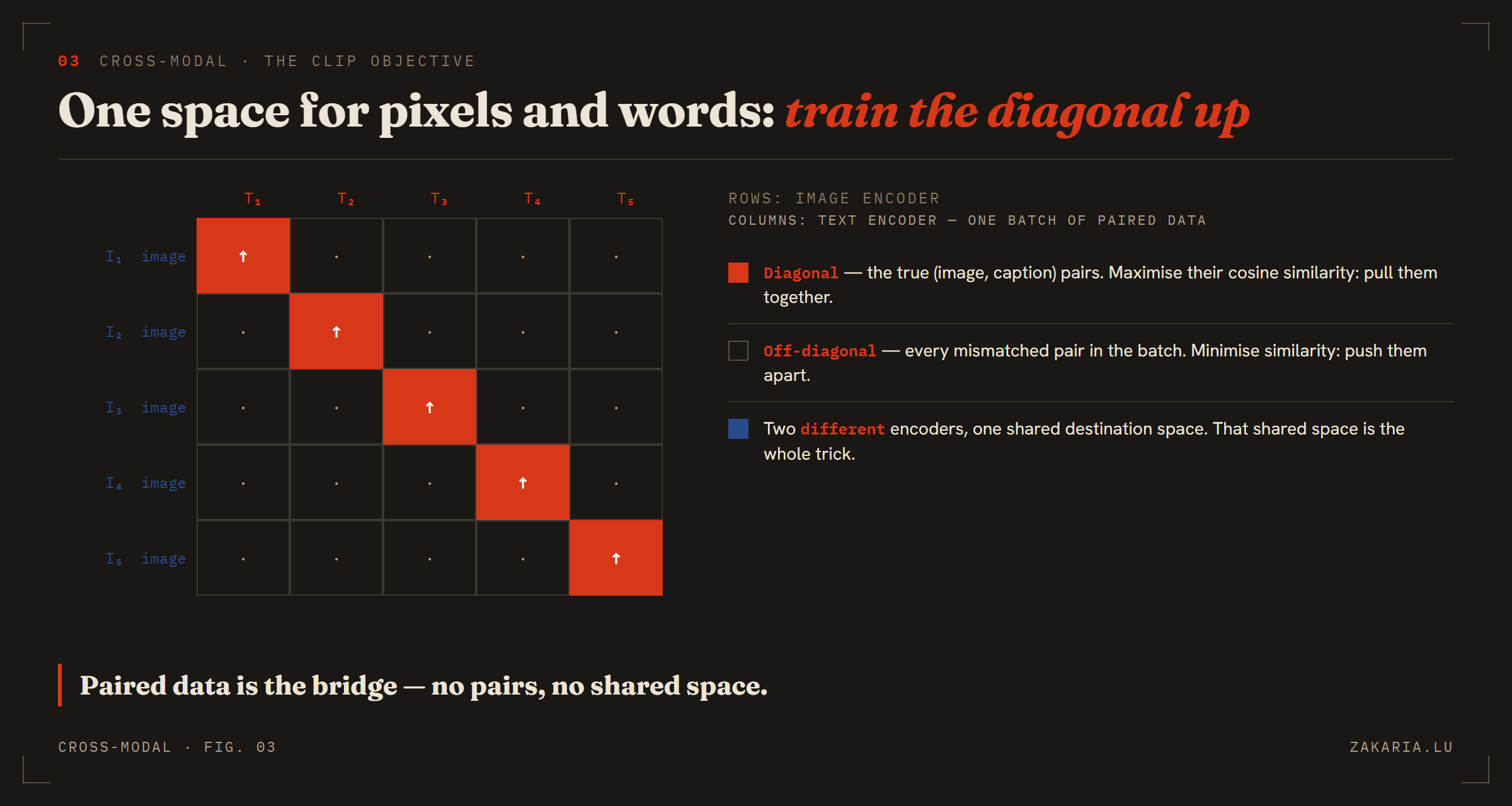
Notice what is and is not shared. The encoders never share weights — a vision transformer and a text transformer are entirely different architectures. What they share is the destination space and the loss that forces both to agree on where things go. This is exactly the mechanism behind zero-shot classification: to label an image, embed it, embed the text "a photo of a {label}" for each candidate, and take the nearest — the same cosine ranking as the script above, now crossing from pixels to words.

Two generalisations are worth naming. First, you can bridge more than two modalities without pairing all of them: ImageBind aligns six modalities using only image-paired data, letting audio and text align through the shared image hub without ever seeing an audio–text pair. Second, when you already hold two frozen, separately trained spaces, you can stitch them with a small learned projection — sometimes literally solving for an orthogonal transform, the classical Procrustes problem. That projection approach is how many multimodal LLMs graft a frozen vision encoder onto a frozen language model: freeze the expensive parts, learn only the bridge.

Practical footnotes

A few things that save time in production. For normalised embeddings, cosine, dot product, and Euclidean distance all induce the same ranking — ‖a - b‖² = 2 - 2(a · b) — so a vector database configured for "cosine" or "dot" returns identical neighbours, and dot is cheaper because it skips the square root. If you swap in a model that does not normalise, a bare dot product silently rewards long vectors; divide by the norms or normalise up front. And retrieval-tuned models such as the bge family expect a short instruction prefix on the query — omitting it quietly costs you recall. These are small details that each cost a real drop in quality when missed.

Where this series goes

This part established the substrate: text becomes arrows, comparison becomes an angle, and a contrastive objective is what arranges the arrows so the angles mean something. Everything more elaborate — attention as a learned, content-dependent similarity; transformers as stacks of such comparisons; retrieval and RAG as nearest-neighbour search over exactly these vectors — is built on this floor. The next part climbs one level up, to how a model turns these static embeddings into contextual ones, where the vector for a word depends on the sentence around it. That is where attention enters.