Self-attention, from scratch: a context vector is a weighted average
I bounced off the maths, then it turned out to be three operations
I'm a backend engineer. I live in Java, Spring, Kafka — types, loops, objects. When I hit chapter 3 of Sebastian Raschka's Build a Large Language Model (From Scratch), the wall of summation signs and the phrase "scaled dot-product attention" did what dense maths always does to me: it slid straight off. Chapter 2 had already been a slog for the same reason — lots of notation, not enough pictures.
So I rebuilt the first attention mechanism the way I wish it had been handed to me: as code, with concrete numbers, one small step at a time. And the punchline is almost annoying. The whole "simplified self-attention" section is three operations a programmer already knows:
Multiply-and-add two lists of numbers — a
forloop withsum += a[i]*b[i]. That's a dot product.Normalise a list so it adds up to 1 — turning raw scores into percentages. That's softmax.
Weighted average of some vectors — multiply-and-add again.
No calculus. No gradients (not yet). If you can write a nested loop, you can write self-attention.
Where this sits: the four rungs of chapter 3
Chapter 3 isn't one mechanism, it's four, each fixing a flaw in the one below it. It helped me enormously to see the whole ladder before climbing, so I stopped expecting rung 1 to already be the thing GPT uses:
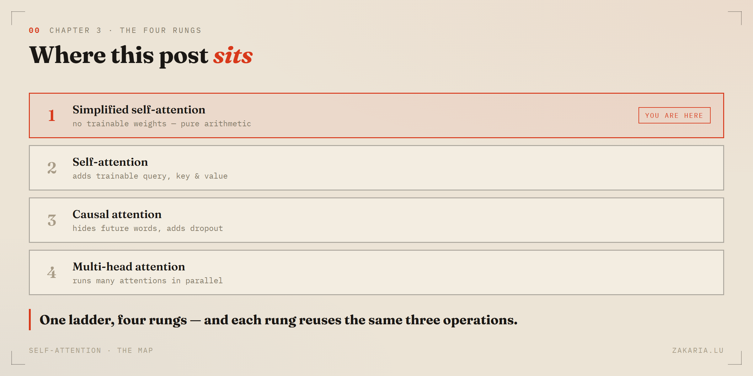
This post is rung 1. It has zero trainable parameters on purpose — it exists to isolate the mechanism before the learning machinery arrives in rung 2.
Every rung reuses the same three operations. Nail them once here and the rest of the chapter is variations on a theme. Here's the spine we're building:
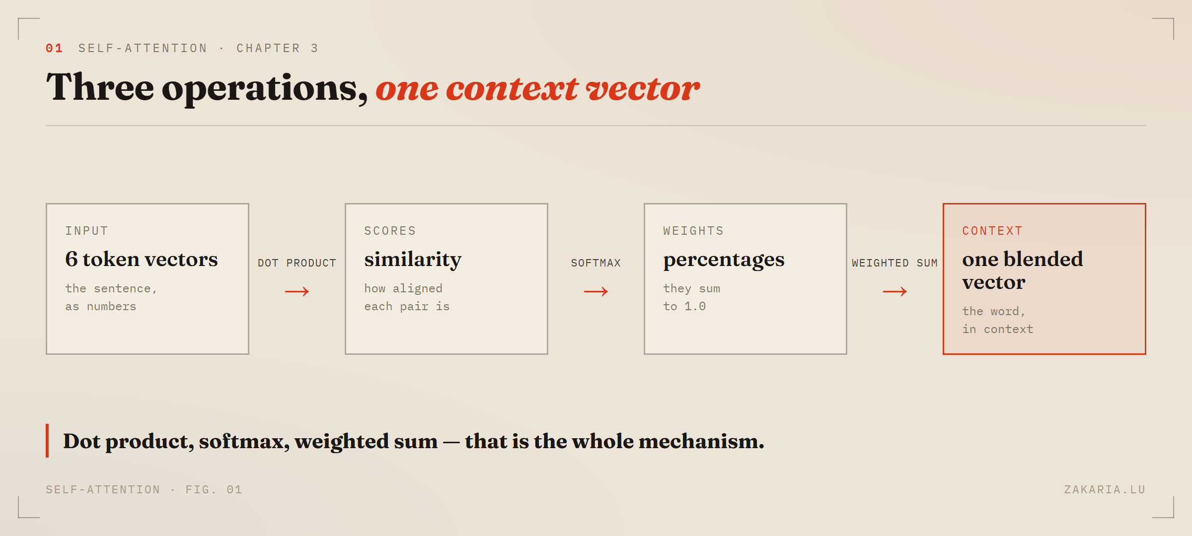
The whole post is this one pipeline. The rest is just filling in each arrow with real numbers.
The one idea: a word becomes a blend of its neighbours
Here's the problem attention solves. A plain embedding gives the word "journey" the same vector no matter what sentence it sits in. But meaning depends on the company a word keeps. Self-attention fixes this: for every word, it builds a new vector — a "context vector" — that is a blend of all the words in the sentence, weighted by how relevant each one is.
In Java terms, a context vector is a weighted average over a List<double[]>:
double[] context = new double[3];
for (int i = 0; i < tokens.size(); i++) {
    for (int d = 0; d < 3; d++) {
        context[d] += weight[i] * tokens.get(i)[d];  // weighted sum
    }
}
The entire chapter is really one question: where do those weight[i] values come from? Here's the answer for the word "journey" in the book's toy sentence, "Your journey starts with one step":
![Six tokens with attention weights as bars; journey 0.24 and starts 0.23 are largest. They sum, arrow, to context vector [0.44, 0.65, 0.57].](/blog/media/7240a4a5589665d4d4550a9af19c250be2fb94e8a2cdcfa259b7d1efa53626cc.png)
The six weights sum to 1.0 — they're just percentages. "journey" spends 24% of its attention on itself, 23% on "starts", 11% on "one".
Do that blend for all six words and you've replaced six context-blind embeddings with six context-aware ones. That's self-attention. Now let's earn those weights from scratch, in three steps.
Step 1 — attention scores are just dot products
Chapter 3 uses six toy tokens, each a 3-number vector (real GPT embeddings have thousands of dimensions, but the mechanism is identical):
Your     [0.43, 0.15, 0.89]
journey  [0.55, 0.87, 0.66]   (our query)
starts   [0.57, 0.85, 0.64]
with     [0.22, 0.58, 0.33]
one      [0.77, 0.25, 0.10]
step     [0.05, 0.80, 0.55]
We pick one word to focus on — "journey" — and score it against every token in the sentence, itself included. The "score" is the dot product of the two vectors: the same measure of alignment behind cosine similarity. One worked example, "journey" against "Your":
0.55*0.43 + 0.87*0.15 + 0.66*0.89
=  0.2365 +  0.1305 +  0.5874  = 0.9544
Do that six times and you get "journey"'s raw scores (the book calls these attn_scores_2):
journey . Your     = 0.9544
journey . journey  = 1.4950   (highest)
journey . starts   = 1.4754   (highest)
journey . with     = 0.8434
journey . one      = 0.7070
journey . step     = 1.0865
Look at why "journey" and "starts" score highest — their vectors are almost identical, so they point the same way, so their dot product is large. The lowest scorer, "one" [0.77, 0.25, 0.10], points in a noticeably different direction. Alignment is attention.
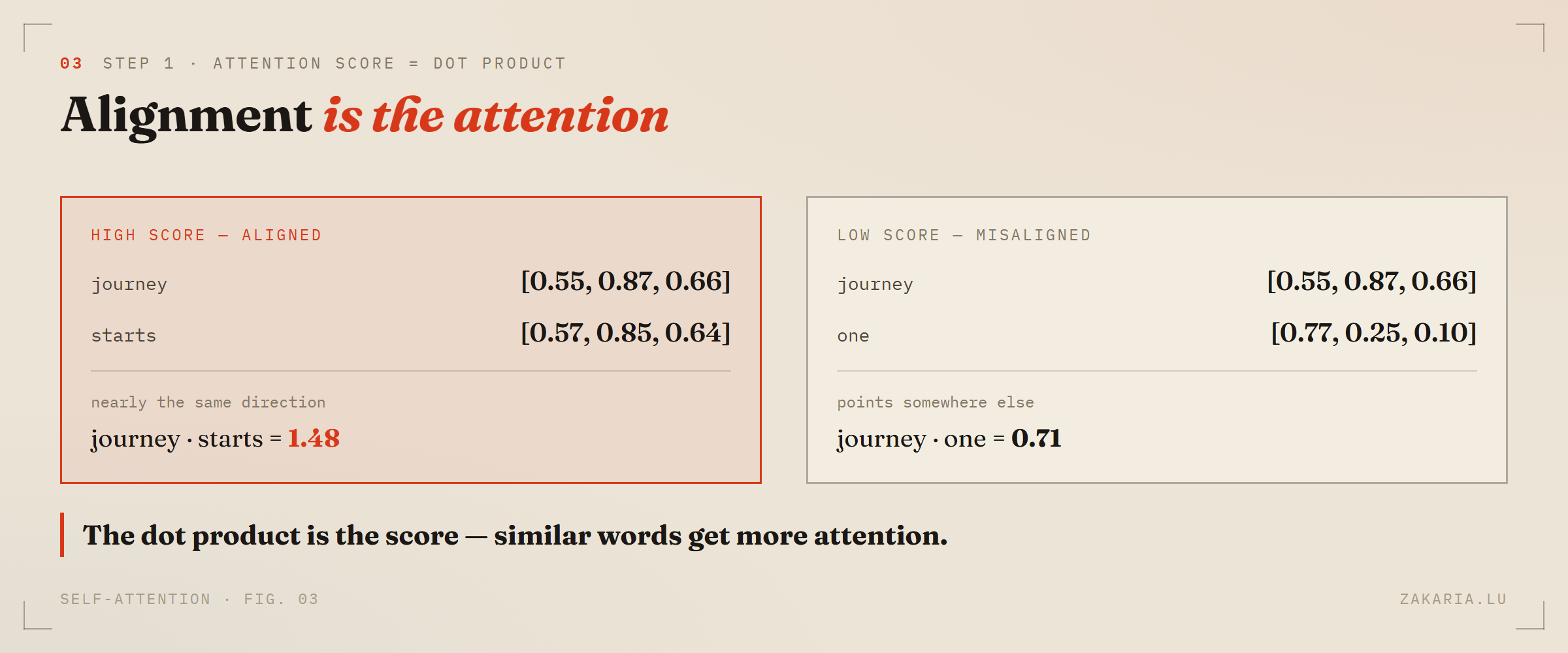
Near-identical vectors score high; vectors pointing elsewhere score low. The dot product is the attention score.
Step 2 — turning scores into weights (my wrong-ish first guess)
The scores are 0.95, 1.50, 1.48, 0.84, 0.71, 1.09, but attention weights need to be percentages that sum to 1.0. When I first hit this, my instinct was the obvious one: divide each score by the total. That is exactly right — and it's literally the book's first attempt (attn_scores / attn_scores.sum()). The six scores add up to 6.56, so:
token      score / 6.56     weight
Your        0.95 / 6.56  =   0.146
journey     1.50 / 6.56  =   0.228
starts      1.48 / 6.56  =   0.225
with        0.84 / 6.56  =   0.128
one         0.71 / 6.56  =   0.108
step        1.09 / 6.56  =   0.166
Those sum to 1.0 and they look reasonable. So why isn't this the real recipe? One catch: dot products can come out negative when two vectors point in opposite directions, and dividing by the sum falls apart the moment that happens. Suppose just two tokens scored 1.5 and -0.4. The total is 1.1, so plain division gives:
score    / sum (= 1.1)     weight
 1.5       1.5 / 1.1  =      1.36    (136%!)
-0.4      -0.4 / 1.1  =     -0.36    (-36%!)
A weight of 136% and a weight of −36% are nonsense — you can't pay negative attention. The naive version only looked fine because our toy scores happened to all be positive.
Softmax: the same idea, hardened
Softmax is your percentage idea with one extra move up front: run every score through exp() first, then divide by the total. exp() maps any number — negative included — to a positive one, so the division always behaves. As a bonus it stretches the gaps, so a bigger score claims a proportionally bigger slice. Watch the same six scores flow through it:
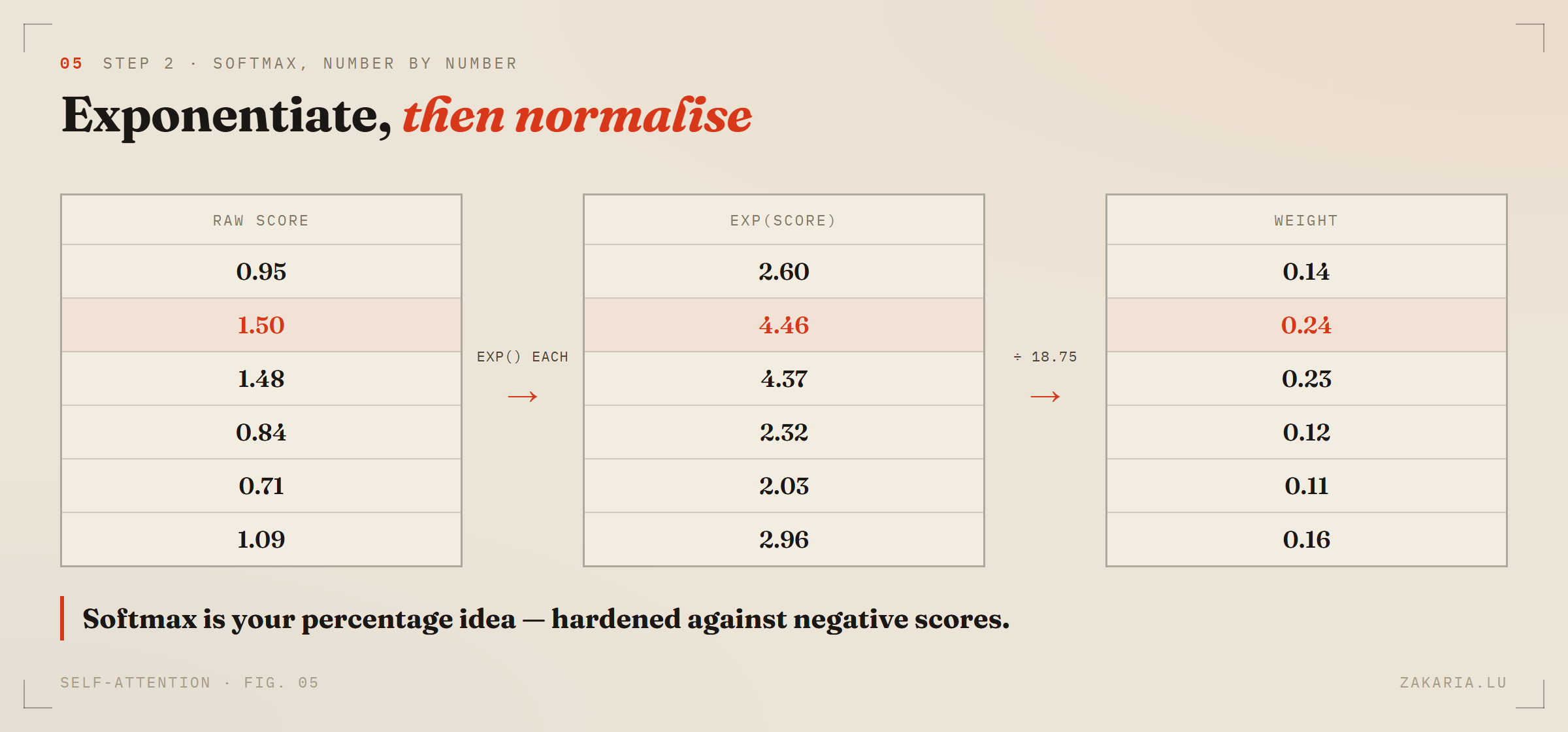
exp() lifts every score positive and widens the gaps; dividing by the column total (18.75) turns them into weights that sum to 1.0.
Those weights — 0.14, 0.24, 0.23, 0.12, 0.11, 0.16 — are exactly the bars from the blend picture earlier. And notice what the exp() did: plain division gave "journey" a 0.228 share; softmax nudged it to 0.238. The biggest score got a slightly bigger slice. That sharpening, plus surviving negatives, is the whole reason softmax wins over my first guess.
Step 3 — the weighted sum
Now we spend the weights. The context vector is each token vector times its weight, all summed — the exact for loop from the top of the post:
z2 = 0.14*Your + 0.24*journey + 0.23*starts + 0.12*with + 0.11*one + 0.16*stepEach token is three numbers, so we do this per column. The first column works out to:
0.14*0.43 + 0.24*0.55 + 0.23*0.57 + 0.12*0.22 + 0.11*0.77 + 0.16*0.05 = 0.4419Do all three columns and "journey"'s context vector is [0.4419, 0.6515, 0.5683]. Sanity-check its shape against the inputs:
journey (original)   [0.55, 0.87, 0.66]
starts  (original)   [0.57, 0.85, 0.64]
z2      (context)    [0.44, 0.65, 0.57]   (pulled toward both)
The result leaned toward "journey" and "starts" — the tokens it paid the most attention to. Exactly what a weighted average should do.
All of it, in three lines of PyTorch
Here's the part that made me feel silly for being intimidated. Everything above — and for all six tokens at once, not just "journey" — is three lines, because a matrix multiply is a batch of dot products:
attn_scores  = inputs @ inputs.T                    # step 1: every pair's dot product (6x6)
attn_weights = torch.softmax(attn_scores, dim=-1)   # step 2: each row becomes percentages
context_vecs = attn_weights @ inputs                # step 3: the weighted blend (6x3)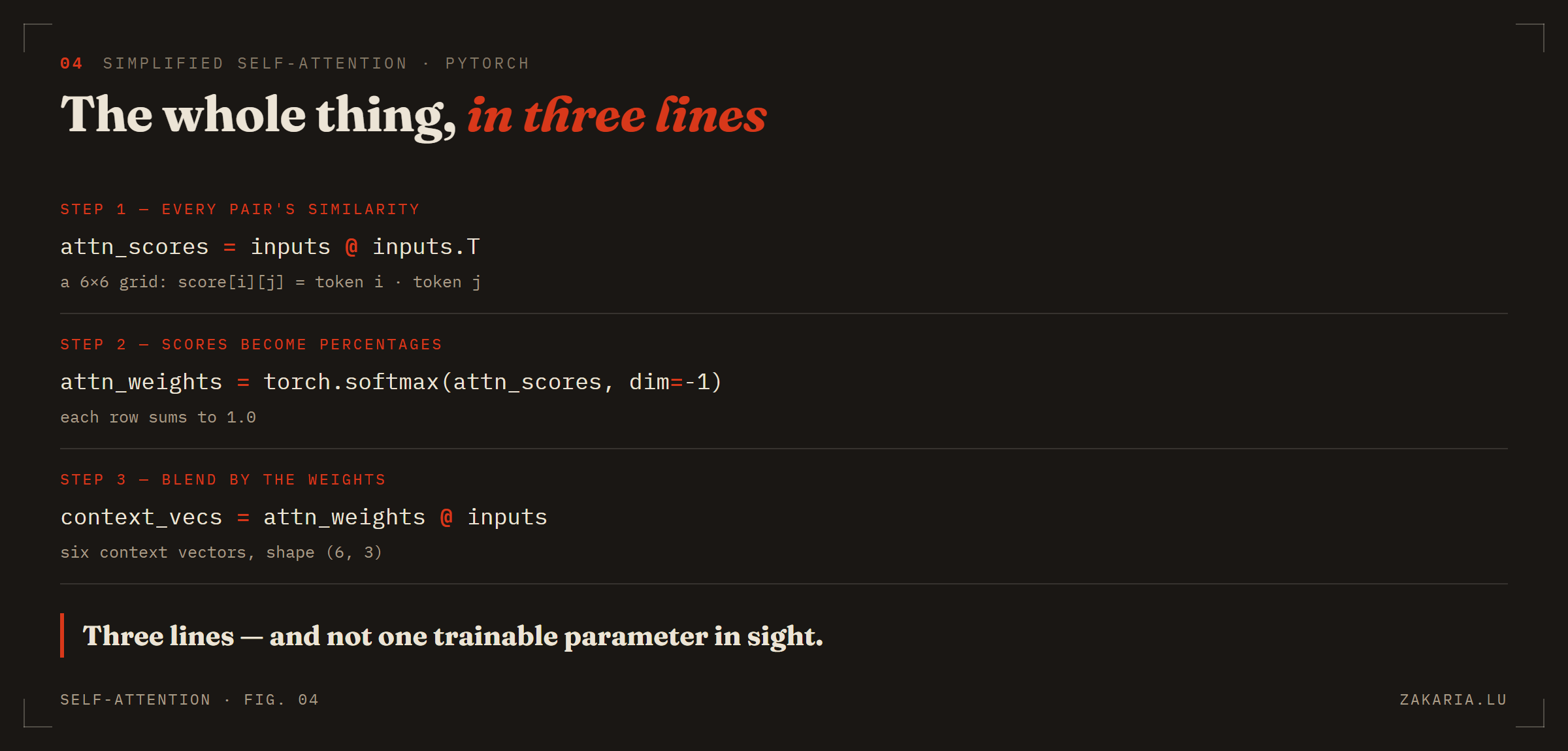
The @ operator is matrix multiplication — a batch of dot products. Three lines, and not one trainable parameter.
Line 1 does what we did for "journey" for every token in one shot: inputs @ inputs.T is a 6×6 grid where cell [i][j] is token i dotted with token j. Line 2 softmaxes each row into weights. Line 3 blends, giving six context vectors of shape (6, 3) — one context-aware vector per word.
The catch: nothing has been learned yet
Read those three lines again and something should nag at you. There are no adjustable knobs. We took the raw input vectors, dotted them against each other, softmaxed, and blended. A neural network is supposed to train — but there isn't a single weight here that gradient descent could nudge.
That's on purpose, and it's why rung 1 is called "simplified". It isolates the mechanism — scores, weights, blend — before adding the machinery that learns. Rung 2 introduces three small trainable matrices, the famous query, key and value projections, which let the model learn what "relevant" should mean instead of reading it straight off the raw embeddings. Same three operations; three learnable knobs bolted on.
One last thing that tripped me up, coming from chapter 2: I kept expecting positional vectors to show up here. They don't. Position is added to the embeddings before attention ever runs, so by the time a token reaches this pipeline, any order information is already baked into its vector. Chapter 3 drops positions entirely from the toy inputs just to keep the spotlight on attention.
Next in the series: trainable self-attention — query, key, value, and the "scaled" in scaled dot-product attention.