Trainable self-attention: query, key, value, and a thermostat on the softmax

Part 6 ended on a confession: the simplified self-attention I had just built had zero parameters. Scores were x · x, raw embedding against raw embedding, so "relevance" was whatever geometry chapter 2's embedding table happened to have. Nothing could learn what relevant means. Section 3.4 of Sebastian Raschka's Build a Large Language Model (From Scratch) fixes that with one move, and this post is that move worked through on my usual six tokens, The cat sat on the mat, with every number printed from real PyTorch output.

The skeleton does not change. It is still scores → softmax → weighted blend. What changes is that each embedding is first pushed through three small learnable matrices, and those three matrices are the only thing training ever touches.

Who owns what: three shared matrices, eighteen private vectors

This is the part I wish I had read first, because I chased it question by question instead. Two kinds of objects exist, and they are owned differently.

• Once, shared, learned: W_query, W_key, W_value. Three matrices. The same three for every token, every sentence, every batch. They are the model's knobs, exactly like the embedding table from part 5.
• Per token, private, computed: each token multiplies its own embedding by those three shared matrices and gets its own q, k, v. Six tokens times three roles is eighteen vectors, and they are thrown away and recomputed for every new sentence.

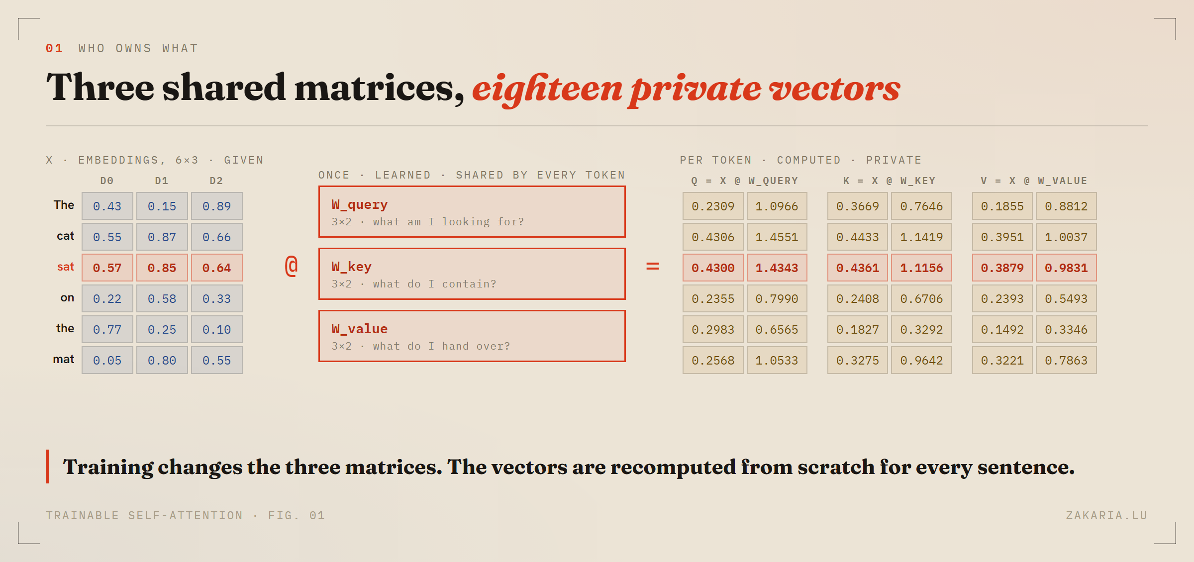
The three roles have names that are worth keeping literal. Think of a library search. The query is what a token is looking for. The key is what a token contains, the index card. The value is what a token hands over if someone decides to look at it, the book itself. You match your query against every key, then walk away with a blend of the values.

import torch, torch.nn as nn

X = torch.tensor([
    [0.43, 0.15, 0.89],   # The
    [0.55, 0.87, 0.66],   # cat
    [0.57, 0.85, 0.64],   # sat
    [0.22, 0.58, 0.33],   # on
    [0.77, 0.25, 0.10],   # the
    [0.05, 0.80, 0.55],   # mat
])
d_in  = X.shape[1]   # 3, forced by the embedding
d_out = 2            # chosen, so the numbers fit on screen

torch.manual_seed(123)
W_query = nn.Parameter(torch.rand(d_in, d_out), requires_grad=False)
W_key   = nn.Parameter(torch.rand(d_in, d_out), requires_grad=False)
W_value = nn.Parameter(torch.rand(d_in, d_out), requires_grad=False)

W_query =
 tensor([[0.2961, 0.5166],
         [0.2517, 0.6886],
         [0.0740, 0.8665]])

d_in is forced, d_out is a choice

The 3 in [3, 2] is not a decision. A row of X has three numbers, and x @ W only multiplies if the length of x equals the number of rows of W: [1×3] @ [3×2] → [1×2]. The two inner threes must match, which is why the code says d_in = X.shape[1] rather than typing a number. GPT-2's embeddings are 768 long, so there d_in = 768.

The 2 is free. It sets how long q, k and v are. I picked 2 so every matrix fits on a screen. GPT-2 picks 768, so d_out = d_in there, but that is a convention, not a rule of the arithmetic.

One token, end to end: sat in five lines

Raschka's discipline is to follow one token through the whole pipeline before touching the matrix version, and it is the right discipline. The query token is sat, row 2 of X.

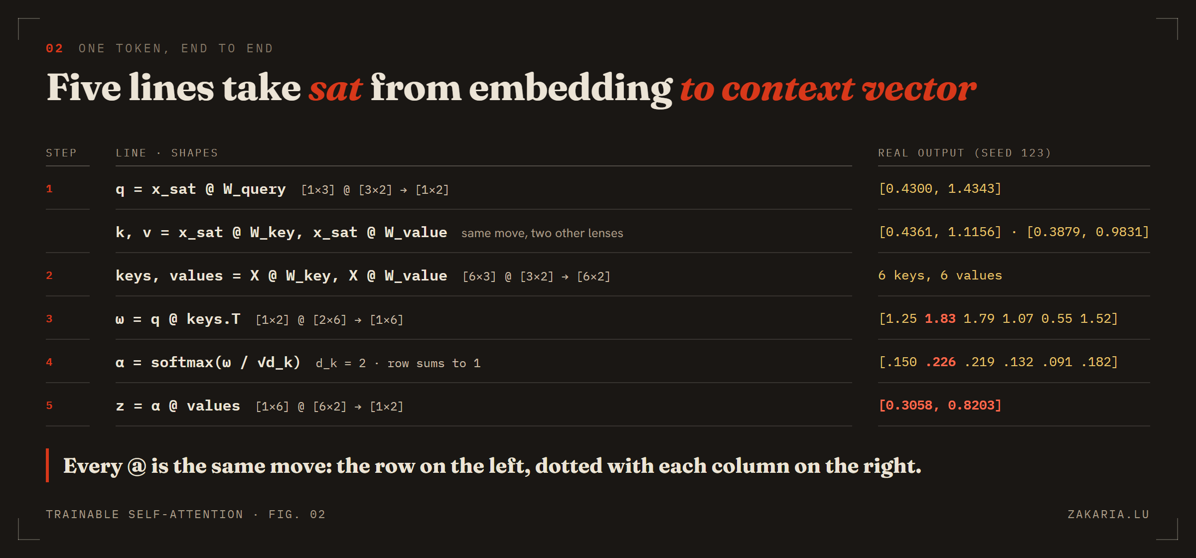
Step 1, project. sat's three numbers go through each matrix and come out as three two-number vectors.

x_sat     = X[2]                 # [0.57, 0.85, 0.64]
query_sat = x_sat @ W_query      # [0.4300, 1.4343]
key_sat   = x_sat @ W_key        # [0.4361, 1.1156]
value_sat = x_sat @ W_value      # [0.3879, 0.9831]

Step 2, everyone gets a key and a value. Only sat is asking, so only sat needs a query right now. But every token must be askable, so all six rows go through W_key and W_value. That is step 1 repeated for six rows, twelve dot products each, laid out as a 6×2 grid.

keys   = X @ W_key      # [6,3] @ [3,2] -> [6,2]
values = X @ W_value    # [6,3] @ [3,2] -> [6,2]

Step 3, score. The same dot product as part 6, but between sat's query and each token's key, not between raw embeddings. The transpose is there so that the keys sit as columns on the right.

attn_scores_sat = query_sat @ keys.T    # [1,2] @ [2,6] -> [1,6]
# The 1.2544  cat 1.8284  sat 1.7877  on 1.0654  the 0.5508  mat 1.5238

Checking the top one by hand: 0.4300 × 0.4433 + 1.4343 × 1.1419 = 1.8284. Same ranking as part 6, cat and sat on top, but now the ranking itself is trainable. Change W_query or W_key and the whole bar chart moves.

Step 4, scale, then softmax. New detail: before softmax, every score is divided by √d_k, where d_k is the length of a key, 2 here.

d_k = keys.shape[-1]                                            # 2
attn_weights_sat = torch.softmax(attn_scores_sat / d_k**0.5, dim=-1)
# The 0.1503  cat 0.2256  sat 0.2192  on 0.1315  the 0.0914  mat 0.1819   sum 1.0000

Step 5, blend the values. Part 6 blended the rows of X. Now each weight multiplies that token's value vector, and the six results are added down each column.

context_sat = attn_weights_sat @ values   # [1,6] @ [6,2] -> [1,2]
# z_sat = [0.3058, 0.8203]

Read that as 15% of The's value plus 23% of cat's value plus 22% of sat's own value and so on. sat went in as three given numbers and came out as a two-number context vector shaped entirely by three learnable matrices.

The @ that tripped me: row on the left, each column on the right

I knew @ as the dot product from the maths posts: pair up the coordinates, multiply, add, one number out. Then x_sat @ W_query returned two numbers and I stalled. The resolution is that a matrix on the right is just several column vectors standing side by side, and @ runs the dot product you already know once per column.

x_sat = [0.57, 0.85, 0.64]

column A of W_query = [0.2961, 0.2517, 0.0740]
column B of W_query = [0.5166, 0.6886, 0.8665]

x_sat . column A = 0.57*0.2961 + 0.85*0.2517 + 0.64*0.0740 = 0.4300
x_sat . column B = 0.57*0.5166 + 0.85*0.6886 + 0.64*0.8665 = 1.4343

x_sat @ W_query  = [0.4300, 1.4343]

Proof, since the point of this series is that nothing gets asserted without running it:

by_hand = torch.tensor([torch.dot(x_sat, W_query[:, 0]),
                        torch.dot(x_sat, W_query[:, 1])])
print(torch.allclose(x_sat @ W_query, by_hand))   # True

The same rule scales all the way up. Vector against vector is one dot product. A [6×3] against a [3×2] is twelve, one per row and column pair. queries @ keys.T is thirty-six. Every @ in this post is "the row on the left, dotted with each column on the right".

Why divide by √d_k

Softmax gets peaky when its inputs are big. Same five scores, once as they are and once multiplied by 8:

s = torch.tensor([0.1, -0.2, 0.3, -0.2, 0.5])
torch.softmax(s,     dim=-1)   # [0.192, 0.143, 0.235, 0.143, 0.287]
torch.softmax(s * 8, dim=-1)   # [0.033, 0.003, 0.162, 0.003, 0.800]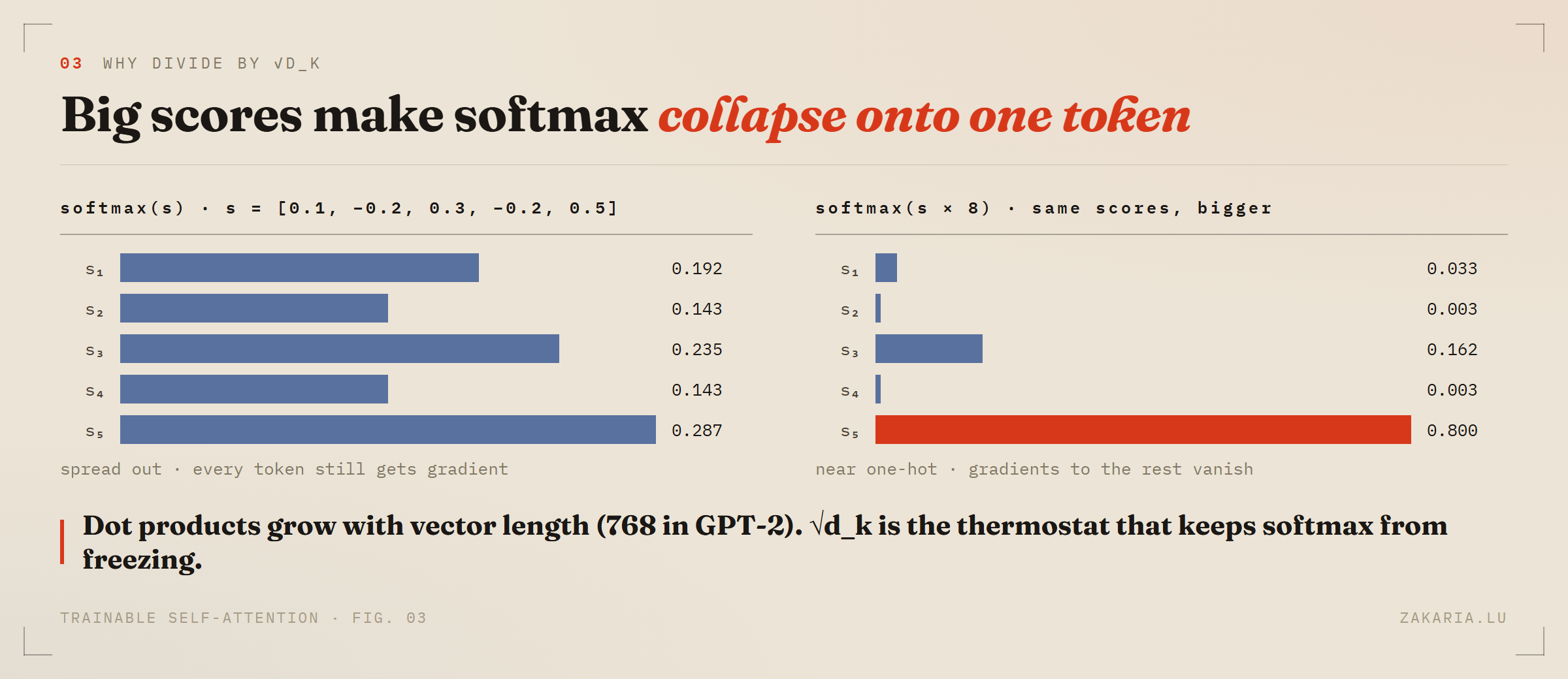

A near one-hot attention row is bad for training, because the tokens that got nothing also get almost no gradient, so nothing about them is learned. Dot products grow with vector length, and GPT-2's are 768 long, so raw scores would be big. Dividing by √d_k keeps them in the range where softmax stays soft. That is the "scaled" in scaled dot-product attention, and the best mental model I have found is a thermostat on the softmax.

"Weights" now means two different things

This one cost me a full round of confusion, and the collision is baked into the vocabulary. In part 6, softmax(X @ X.T) produced a 6×6 matrix I called the attention weights. The new W_query, W_key, W_value are also called weights. They are not the same kind of object.

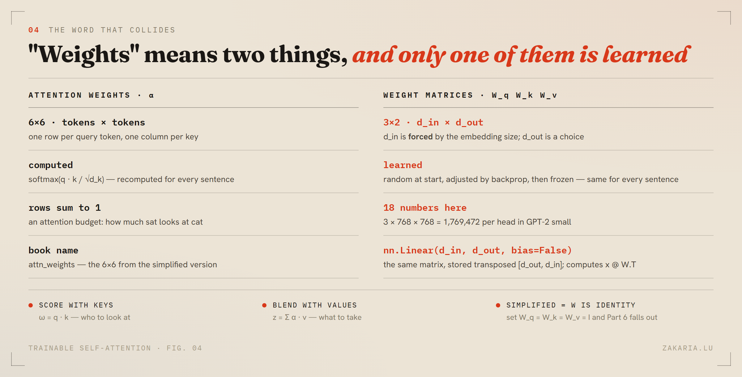
	attention weights α	weight matrices W_q W_k W_v
shape	6×6, tokens × tokens	3×2, d_in × d_out
comes from	computed, softmax(q · k / √d_k)	learned by backprop, random at start
per sentence?	recomputed every time	fixed after training
rows sum to 1?	yes, it is an attention budget	no, just numbers
book name	attn_weights	W_query, W_key, W_value

They relate in one direction: the matrices produce the vectors, the vectors produce the weights. W_q, W_k → q, k → scores → α → z = α @ V. In my own scripts I renamed the 6×6 from part 6 to A so the two never share a letter again.

Which also answers a question I had: is the simplified version ever used? No. But it is not a different algorithm either. Set W_q = W_k = W_v = I, the identity, and q = k = v = x, so part 6 is exactly part 7 with the knobs removed. Its three lines run millions of times inside every GPT layer.

All tokens at once, as a module

Replace x_sat by the whole X and each of the five lines becomes the matrix version of itself. The book wraps it in an nn.Module so the three matrices are registered as trainable parameters.

class SelfAttention_v1(nn.Module):
    def __init__(self, d_in, d_out):
        super().__init__()
        self.W_query = nn.Parameter(torch.rand(d_in, d_out))
        self.W_key   = nn.Parameter(torch.rand(d_in, d_out))
        self.W_value = nn.Parameter(torch.rand(d_in, d_out))

    def forward(self, x):
        queries = x @ self.W_query          # [6,2]
        keys    = x @ self.W_key            # [6,2]
        values  = x @ self.W_value          # [6,2]
        attn_scores  = queries @ keys.T     # [6,6], row i = token i vs every key
        attn_weights = torch.softmax(attn_scores / keys.shape[-1]**0.5, dim=-1)
        return attn_weights @ values        # [6,2]

torch.manual_seed(123)
sa_v1 = SelfAttention_v1(d_in, d_out)
print(sa_v1(X))

The  [0.2996, 0.8053]
cat  [0.3061, 0.8210]
sat  [0.3058, 0.8203]     # identical to the by-hand z_sat
on   [0.2948, 0.7939]
the  [0.2927, 0.7891]
mat  [0.2990, 0.8040]

The sat row matches step 5 to the digit, because row 2 of the 6×6 is exactly the α computed by hand. dim=-1 is load-bearing: normalise across each row, the keys a query looks at, never down a column.

v2: the same machine through nn.Linear

SelfAttention_v2 swaps each nn.Parameter(torch.rand(...)) for nn.Linear(d_in, d_out, bias=False). With no bias, a Linear layer is a matrix multiply. Two practical differences: it stores its matrix transposed, [d_out, d_in], and it initialises with a scheme that trains more stably than uniform random. Different random numbers, so different output, sat → [-0.0749, 0.0702] with seed 789.

class SelfAttention_v2(nn.Module):
    def __init__(self, d_in, d_out, qkv_bias=False):
        super().__init__()
        self.W_query = nn.Linear(d_in, d_out, bias=qkv_bias)
        self.W_key   = nn.Linear(d_in, d_out, bias=qkv_bias)
        self.W_value = nn.Linear(d_in, d_out, bias=qkv_bias)

    def forward(self, x):
        queries, keys, values = self.W_query(x), self.W_key(x), self.W_value(x)
        attn_scores  = queries @ keys.T
        attn_weights = torch.softmax(attn_scores / keys.shape[-1]**0.5, dim=-1)
        return attn_weights @ values

# Exercise 3.1: copy v2's weights, transposed, into v1
sa_v1.W_query.data = sa_v2.W_query.weight.T.clone()
sa_v1.W_key.data   = sa_v2.W_key.weight.T.clone()
sa_v1.W_value.data = sa_v2.W_value.weight.T.clone()
print(torch.allclose(sa_v1(X), sa_v2(X)))            # True
print(sum(p.numel() for p in sa_v2.parameters()))    # 18

Exercise 3.1 is the proof that v1 and v2 are one machine: copy v2's weights into v1 with a .T and the outputs are identical. Eighteen trainable numbers in this toy. For one head of GPT-2 small it is 3 × 768 × 768 = 1,769,472.

requires_grad=False is a print trick, not a design decision

The walkthrough at the top sets requires_grad=False on matrices that are supposedly the whole point of training. That looked wrong to me. It is there only to keep printed output clean: any tensor computed from a trainable parameter carries a grad_fn tag, and the walkthrough prints every intermediate.

x_sat @ W_off   # tensor([0.4300, 1.4343])
x_sat @ W_on    # tensor([0.4300, 1.4343], grad_fn=<SqueezeBackward4>)

for name, p in SelfAttention_v1(3, 2).named_parameters():
    print(name, p.requires_grad)   # W_query True, W_key True, W_value True

Same numbers either way. The real classes leave the default True, so backprop records every operation and training can turn the knobs.

What I would tell myself before starting

• The skeleton is unchanged: score, softmax, blend. Three learned matrices are the only addition.
• Matrices are shared and trained. Vectors are private and recomputed per sentence.
• d_in is forced by the embedding. d_out is a choice.
• Score with keys, blend with values. Never mix the two jobs.
• Scale by √d_k, then softmax. It is a thermostat, not a formality.
• "Weights" is two words. α is computed, W is learned.
• Every @ is the row on the left dotted with each column on the right.

Right now sat attends to mat, a token that has not been written yet. A language model predicts the next token, so it must never peek ahead. Next in the series: causal attention, the mask above the diagonal, the -inf before softmax trick, dropout on the attention weights, and then multiple heads.