How One Weight Learns: Derivatives, Gradients, and the First Update

After cross-entropy and perplexity, I could put a number on a model's prediction error. The next question was more practical: how does that number tell a weight what to do?

I want to follow one update completely: choose a tiny model, calculate its loss, find a derivative, and change one weight. Every value below is either supplied, calculated, or explicitly chosen.

One input, one target, one adjustable number

My model multiplies an input by a weight:

prediction = w × x

x = 2       supplied input
target = 6  supplied expected answer
w = 1       chosen starting weight

The prediction is 1 × 2 = 2, but the target is 6. Only w can change. The input and target stay fixed. These are individual numbers: scalar values, with no batch or vocabulary dimension.

For this teaching example I use squared error:

L(w) = (prediction − target)²
     = (2w − 6)²

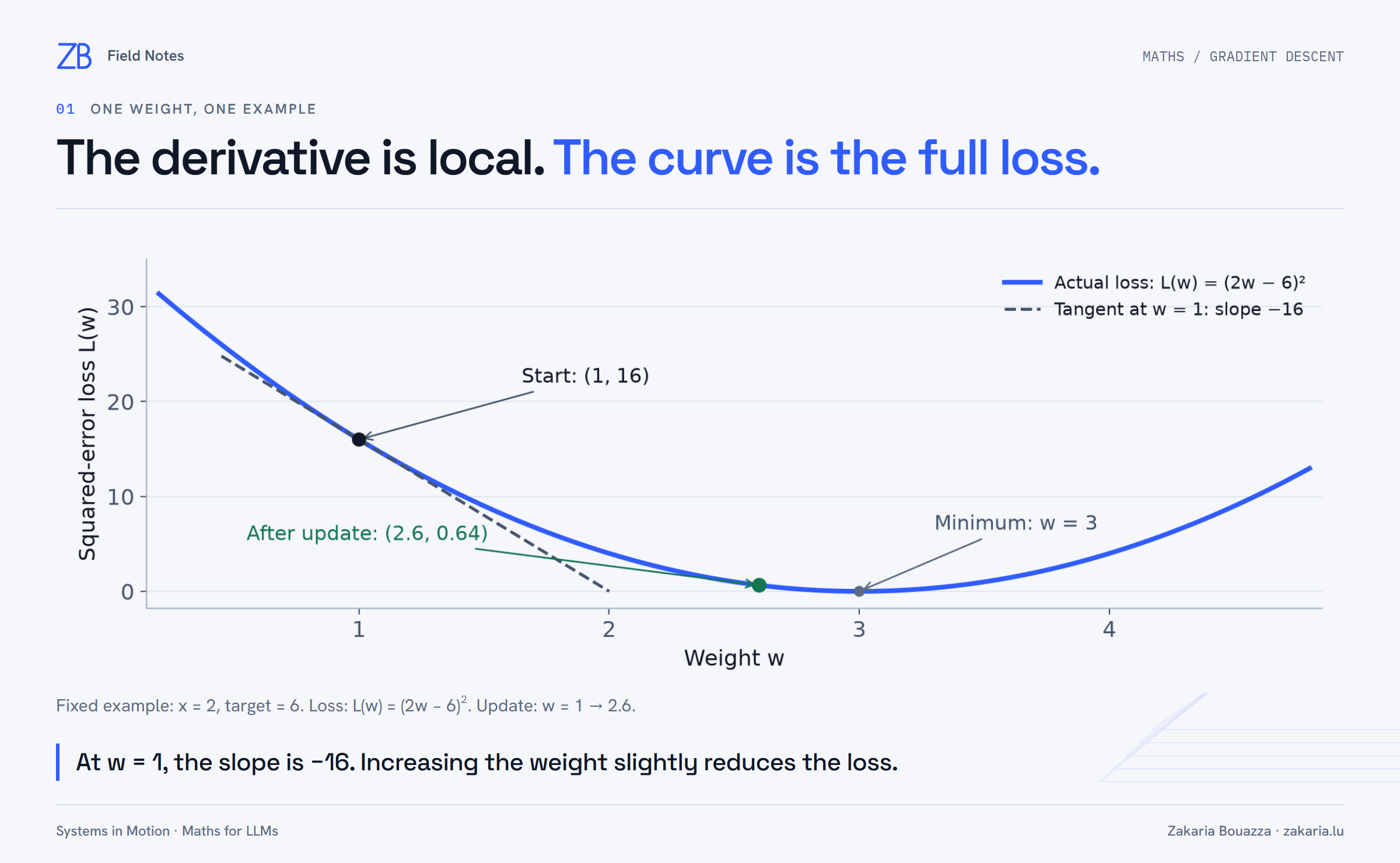
L(1) = (2 − 6)² = 16

L names the loss function; L(w) means “the loss calculated using weight w.” Squaring makes positive and negative errors contribute non-negative losses. This is a small regression example. GPT's next-token objective uses cross-entropy; I am simplifying the objective to expose the update mechanics.

A derivative measures a local change

A loss of 16 tells me how bad this prediction is under my chosen objective. It does not tell me whether to increase or decrease the weight. To investigate, I increase w by a small amount, called h:

h = 0.01
new weight = 1.01
L(1.01) = (2 × 1.01 − 6)² = 15.8404

change in loss / change in weight
= (15.8404 − 16) / 0.01
= −15.96

The negative sign says the loss decreased when the weight increased. The quotient measures loss change per unit of weight change; the actual loss change here is −0.1596.

This quotient is an average slope across a small interval. The derivative is the value it approaches as that interval shrinks toward zero. At this weight, nudges of 0.1, 0.01, and 0.001 give slopes −15.6, −15.96, and −15.996. They approach −16.

Find the exact slope without guessing smaller nudges

The notation dL/dw means “the derivative of loss with respect to weight.” We can calculate it by expanding the square. For a nonzero nudge h:

L(w + h) = (2w − 6 + 2h)²
         = (2w − 6)² + 4h(2w − 6) + 4h²

[L(w + h) − L(w)] / h
= 4(2w − 6) + 4h

As h approaches zero, 4h approaches zero. The remaining expression is the exact derivative:

dL/dw = 4(2w − 6) = 8w − 24

At w = 1:  dL/dw = 8 − 24 = −16

We never divide by zero. We simplify the quotient for nonzero nudges, then examine its limit. The derivative describes the slope here, not a guarantee about arbitrarily large moves.

From derivative to gradient to update

With several weights, the gradient collects one partial derivative for each weight, measuring its local effect while holding the others fixed. Our model has only one weight, so its gradient has one component: −16.

Basic gradient descent subtracts a scaled gradient:

new weight = old weight − learning rate × gradient

learning rate = 0.1
new weight = 1 − 0.1 × (−16) = 2.6

The learning rate is a positive step-size setting I choose. Subtracting a negative gradient increases the weight; subtracting a positive gradient decreases it. This moves opposite the local direction of increasing loss.

Now I run the forward calculation again:

new prediction = 2.6 × 2 = 5.2
new loss = (5.2 − 6)² = 0.64

The loss fell from 16 to 0.64. The exact best weight for this example is 3, because 3 × 2 = 6. One update moved closer; it did not solve the example perfectly.

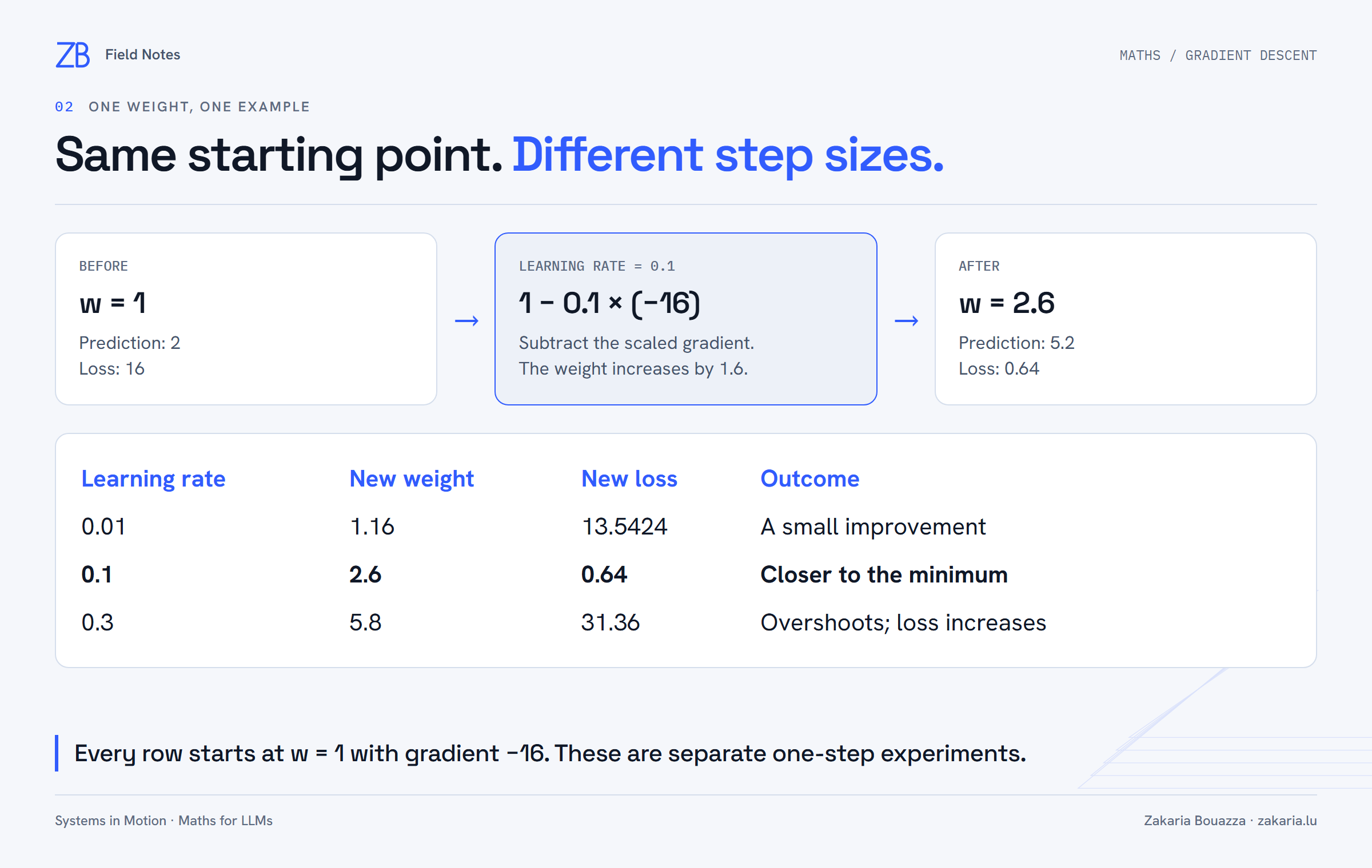
For example, choosing learning rate 0.3 gives w = 5.8 and loss 31.36: worse than the starting loss. The gradient supplied a useful local direction, but the step was too large.

Verify the same update in PyTorch

This example uses ordinary SGD with no momentum or weight decay, matching our arithmetic. It does not claim to reproduce AdamW's update rule.

import torch

x = torch.tensor(2.0)
target = torch.tensor(6.0)
w = torch.tensor(1.0, requires_grad=True)
optimizer = torch.optim.SGD([w], lr=0.1)

optimizer.zero_grad()
prediction = w * x
loss = (prediction - target) ** 2
loss.backward()

print(w.item(), w.grad.item())  # 1.0, -16.0
optimizer.step()

with torch.no_grad():
    new_loss = (w * x - target) ** 2

print(f"w={w.item():.6f}, loss={new_loss.item():.6f}")
# w=2.600000, loss=0.640000

requires_grad=True lets PyTorch record the operations needed to differentiate the loss with respect to w. backward() computes and stores the derivative in w.grad; the weight is still 1. optimizer.step() changes it. PyTorch uses differentiation rules through the recorded operations, not the finite nudges I used to introduce the slope. See its autograd explanation and SGD reference.

zero_grad() clears old gradients because backward calls accumulate them. For another training step, clear them again and recompute the loss at the new weight. The old gradient describes the old position.

That is the bridge from my loss and perplexity article to learning: evaluate the current prediction, calculate how parameters affect its loss, then apply an update. Backpropagation extends the derivative calculation through many connected operations. Here, one weight is enough to see what actually changes.