Cross-Entropy: Understanding the Minus, the Log, and the Loss

Cross-entropy looked difficult to me. Even before getting to the calculation, there was a name to decode, a logarithm, a minus sign, and a formula with a big summation symbol.

I want to build it from one question: how much probability did the model give the correct next token? Everything below starts there.

Start with one correct token

Imagine a tiny vocabulary containing only tea, coffee, and rain. Each word is one token in this toy example. The training text says “I drink tea”, so after “I drink”, our target is tea.

Token	Predicted probability	Target
tea	0.70	1
coffee	0.20	0
rain	0.10	0

The probabilities add to 1. The target column is a one-hot distribution: 1 for the observed answer and 0 elsewhere. It describes this training example; it does not claim that “coffee” is impossible in ordinary language.

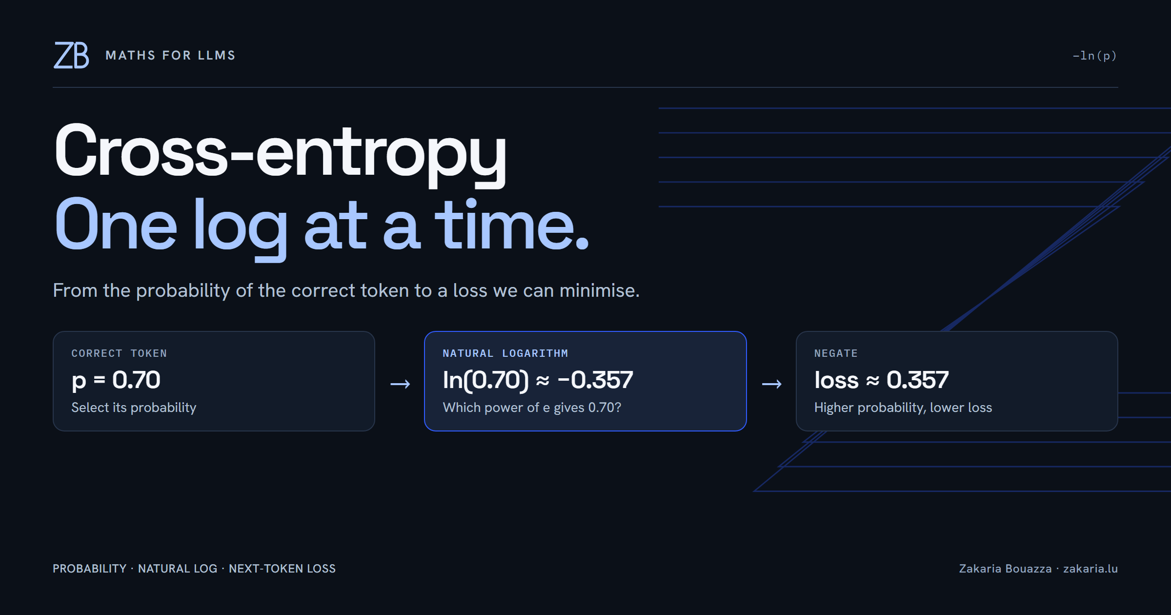
Call the model’s probability for the correct token p. Here, p = 0.70. We want a loss, a number to minimise, that gets smaller as that probability gets larger. For this example, cross-entropy is:

loss = −ln(p)
     = −ln(0.70)
     ≈ 0.357

What does ln actually mean?

A logarithm reverses exponentiation. Because 2³ = 8, we have log₂(8) = 3: what power of 2 produces 8?

The natural logarithm, written ln, asks the same question using e ≈ 2.71828 as its base. In Python, math.log and torch.log use this natural logarithm.

e⁰ = 1           → ln(1) = 0
e⁻¹ ≈ 0.367879    → ln(0.367879) ≈ −1
e⁻² ≈ 0.135335    → ln(0.135335) ≈ −2

A negative exponent means taking a reciprocal: e⁻¹ = 1/e. That is why numbers between 0 and 1 have negative natural logarithms. Specifically, e^(-0.356675) ≈ 0.70, so ln(0.70) ≈ −0.356675. No hidden operation: we are asking which exponent produces our probability.

Why the minus sign?

For 0 < p ≤ 1, ln(p) is non-positive. Negating it gives a non-negative loss. It also turns maximising log-probability into minimising loss.

Correct-token p	ln(p)	−ln(p)
1.00	0	0
0.90	−0.105	0.105
0.50	−0.693	0.693
0.10	−2.303	2.303
0.01	−4.605	4.605

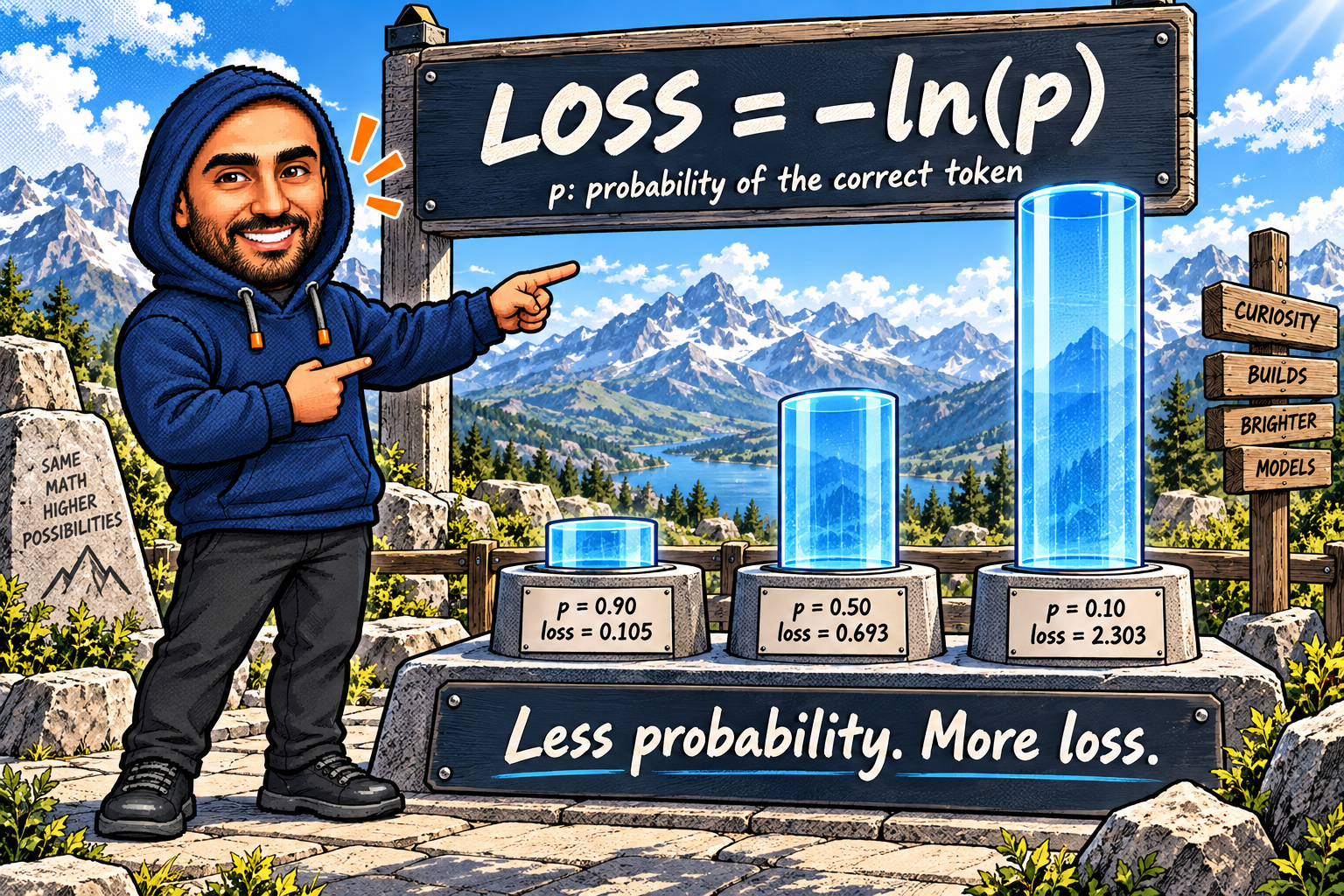
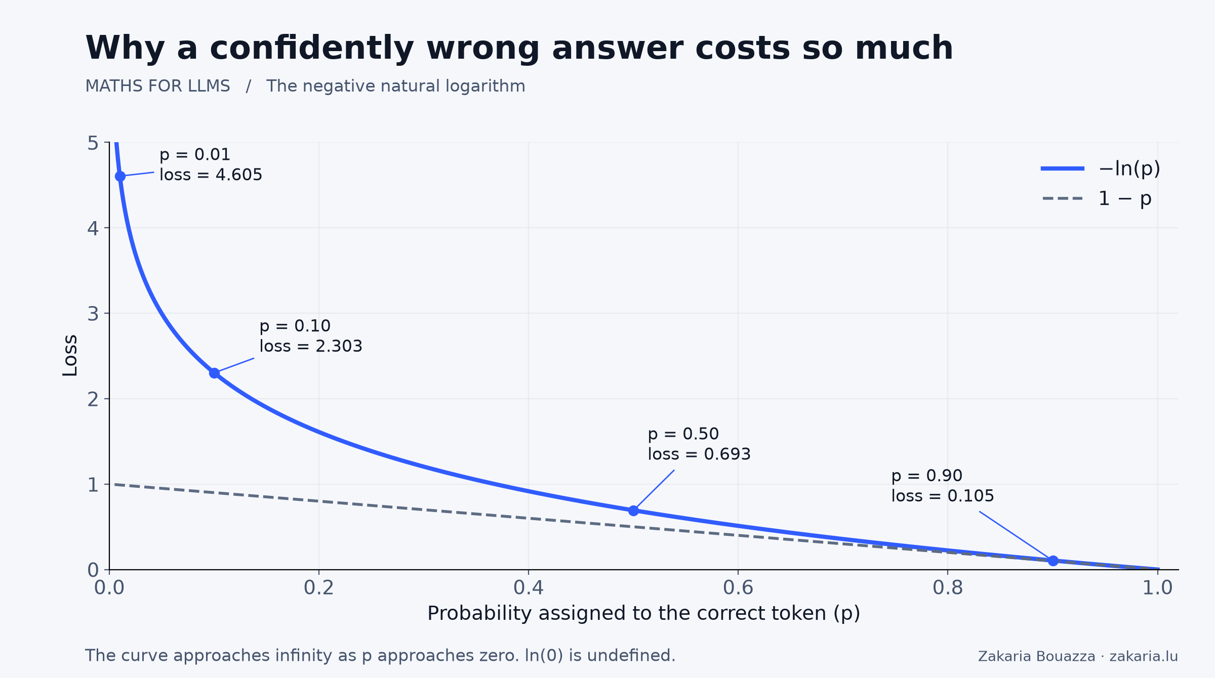
As p approaches zero, the loss grows without bound. ln(0) is undefined; we describe the limiting loss as positive infinity. A confident wrong prediction is expensive because it leaves very little probability for the correct answer.

Why a logarithm instead of 1 − p?

1 − p also decreases when the correct answer gets more probability. But it stays bounded by 1. The logarithmic loss continues growing: reducing p from 0.10 to 0.01 adds about 2.303 to the loss. Another tenfold reduction adds another 2.303.

Logs also turn multiplication into addition. For a sequence, multiply each observed token’s probability conditional on its preceding context. Maximising that product means making the observed sequence more probable:

sequence probability = p₁ × p₂ × p₃
−ln(p₁ × p₂ × p₃) = −ln(p₁) − ln(p₂) − ln(p₃)

This is the negative log-likelihood. The conditional probabilities need not be independent. Working in log space also avoids directly multiplying many tiny probabilities.

Now the full cross-entropy formula

Let qᵢ be the target probability for vocabulary entry i, and pᵢ the model’s predicted probability for that same entry. The symbol Σ means “add over all vocabulary entries”.

H(q, p) = −Σᵢ qᵢ ln(pᵢ)

q = [1,    0,    0   ]
p = [0.70, 0.20, 0.10]

H(q, p) = −[1 × ln(0.70) + 0 × ln(0.20) + 0 × ln(0.10)]
        = −ln(0.70)
        ≈ 0.357

The zeros remove the other terms. That is why a one-hot target reduces the whole formula to the correct token’s negative log-probability. With soft targets, several entries contribute.

Entropy H(q) averages −ln(qᵢ) under q itself. Cross-entropy H(q, p) still averages under q, but scores using another distribution, p. This is where the “cross” comes from. Natural logs measure these quantities in nats; base-2 logs use bits.

From one token to a training loss

Suppose three prediction positions assign their respective correct tokens probabilities 0.80, 0.50, and 0.10. These are three separate predictions, so these numbers need not sum to 1.

mean loss = [−ln(0.80) − ln(0.50) − ln(0.10)] / 3
          ≈ (0.223144 + 0.693147 + 2.302585) / 3
          ≈ 1.072959

For ordinary unweighted next-token training, average over the positions included in the loss, excluding masked or ignored positions. A lower loss means the model assigns higher geometric-mean probability to the observed targets; it does not guarantee every prediction improved.

Check the maths in PyTorch

Logits are the model’s raw scores before softmax. Here we choose [2, 1, 0] to make a runnable example; these produce different probabilities from the earlier table.

import torch
import torch.nn.functional as F

# One prediction, three vocabulary entries: tea, coffee, rain.
logits = torch.tensor([[2.0, 1.0, 0.0]])  # shape (1, 3)
target = torch.tensor([0])               # tea is index 0

probabilities = torch.softmax(logits, dim=-1)
manual = -torch.log(probabilities[0, 0])
loss = F.cross_entropy(logits, target)

print(probabilities)  # tensor([[0.6652, 0.2447, 0.0900]])
print(f"{manual.item():.6f}")  # 0.407606
print(f"{loss.item():.6f}")    # 0.407606
torch.testing.assert_close(manual, loss)

The shape (1, 3) means one prediction over three vocabulary entries. The target [0] selects tea. Softmax converts scores to probabilities; indexing selects the correct one; the negative log scores it.

Pass raw logits to F.cross_entropy. It combines log-softmax with negative log-likelihood for class-index targets, using a numerically stable calculation. Passing softmax probabilities would make it treat those probabilities as new scores. See the PyTorch cross-entropy documentation.

The formula now reads as three concrete actions: select the correct token’s probability, take its negative natural logarithm, then average across the training positions.

Perplexity: undo the log to read the loss differently

Cross-entropy gives us an average negative log-probability. Perplexity takes that same number and applies the exponential function:

perplexity = exp(mean cross-entropy)
           = e^(mean cross-entropy)

Here, exp(x) means e raised to the power x. This formula assumes natural logarithms and the ordinary, unweighted average negative log-likelihood of the observed tokens. If the loss uses base-2 logs, use 2^loss instead.

Why does exponentiating help?

Start with a single correct-token probability p. The exponential reverses the logarithm, and the minus sign turns the result into a reciprocal:

exp(−ln(p)) = exp(ln(1/p)) = 1/p

p = 0.50 → loss ≈ 0.693 → perplexity = 2
p = 0.10 → loss ≈ 2.303 → perplexity = 10

For several tokens, we exponentiate the mean loss. Let N be the number of scored positions, and p₁, …, pₙ their observed-token probabilities. Using the log-of-a-product rule from above:

perplexity = exp(−[ln(p₁) + … + ln(pₙ)] / N)
           = 1 / (p₁ × … × pₙ)^(1/N)

The denominator is the geometric mean: multiply the probabilities, then take the Nth root. Perplexity is its reciprocal. In our three-position example:

geometric mean = (0.80 × 0.50 × 0.10)^(1/3)
               ≈ 0.342
perplexity     = exp(1.072958608…)
               ≈ 2.924

What does “2.924 choices” mean?

If a predictor assigns probability 1/K to every observed target, as a uniform predictor over K possible tokens would, its loss is ln(K) and its perplexity is K. This gives us the intuition of an effective number of equally likely choices.

A perplexity of 2.924 describes the same average log-loss as that effective choice count. It does not mean the model literally considered exactly three tokens or predicted uniformly. Real distributions vary at every position, and tokens are not necessarily whole words.

For the larger loss 10.7940, the calculation is:

perplexity = exp(10.7940)
           ≈ 48,727.56
           ≈ 48,728

That corresponds to a geometric-mean observed-token probability of about 1/48,728. It does not by itself prove that the model is untrained or guessing randomly. Perplexity can even exceed vocabulary size if the model gives the observed tokens less probability than a uniform predictor would.

Compute it, then compare like with like

import torch

# Probabilities of the observed tokens at three prediction positions.
correct_token_probs = torch.tensor([0.80, 0.50, 0.10], dtype=torch.float64)
mean_loss = -torch.log(correct_token_probs).mean()
perplexity = torch.exp(mean_loss)

print(f"{mean_loss.item():.6f}")   # 1.072959
print(f"{perplexity.item():.6f}")  # 2.924018

Average the token losses first, then exponentiate once; averaging individual token perplexities gives a different result. Across batches of different lengths, weight by the number of scored tokens. Exclude padding and ignored positions consistently. Do not blindly exponentiate a sum, a class-weighted loss, or a label-smoothed training objective and call it standard perplexity.

Lower perplexity means higher geometric-mean probability for the observed targets. It is not an accuracy percentage or a guarantee of factual answers. Compare scores on the same evaluation text, tokenizer, and context protocol; changing tokenization or available context changes the score. The Hugging Face perplexity guide explains these evaluation details.

Cross-entropy and perplexity therefore express the same underlying evaluation on different scales: average negative log-probability, and its exponential.